6.2 – Ratios and probabilities
Introduction
One common objective of a research project is comparison between quantities: one effective way to communicate a comparison is to construct a ratio. Ratios provide a standardized way to compare different data sets. The purpose of this page is introduce the wealth of types of ratios used for quantification of comparisons, from indexes to ratios.
Let’s review our definitions again. An event is some occurrence. As you know, a ratio is one number, the numerator, divided by another called the denominator. A proportion is a ratio where the numerator is a part of the whole. A rate is a ratio of the frequency of an event during a certain period of time. A rate may or may not be a proportion, and a ratio need not be a proportion, but proportions and rates are all kinds of ratios. If we combine ratios, proportions, and/or rates, we construct an index.
Ratios
Yes, data analysis can be complicated, but we start with this basic idea. Much of the statistics is based on frequency measures, eg, ratios, rates, proportions, indexes, and scales.
Ratios are the association between two numbers, one random variable divided by another. Ratios are used as descriptors and the numerator and denominator do not need to be of the same kind. Business and economics are full of ratios. For example, return on investment (ROI), eg, earnings equals net income divided by number of shares outstanding, the Price-Earnings, or P/E ratio, is the ratio of the price of a stock to the earnings per stock, as well as many others are used to summarize performance of a business, and to compare performance of one business against another.
Note 1: ROI also stands for region of interest — a sample in a data set identified by the analyst for a particular interest. Often refers to a specific area in an image.
Ratios are deceptively convenient way to standardize a variable for comparisons, ie, how many times one number contains another. For example, when estimating bird counts for different areas, or different birding effort (intensity, time searched), we may correct counts by accounting for area in which counts were made or the total time spent counting, for a per-unit ratio (Liermann et al 2004).
Practice: There were 1,326 day undergraduate students enrolled in 2014 at Chaminade University of Honolulu and the Sullivan Library added 8469 new items (ebooks, journals, etc,) to its collection during 2014. What is the ratio of new items per student?

Data collected from Chaminade University website at www.chaminade.edu on 3 July 2014.
Practice: For another example, what is ratio of annual institutional aid a student at Chaminade University may expect to receive compared to a student at Hawaii Pacific University?

Thus, in 2014, Chaminade offered more than twice the institutional aid to its students then does HPU (both institutions are private universities, data from retrieved on 3 July 2014 from www.cappex.com).
Relative change, Fold-change and orders of magnitude
It’s common practice to report on the amount of change between two quantities recorded over time. Relative change (often percentage) describes change relative to an initial value. Relative change in root length b
To make percent increase (decrease), simply multiple 100%.
(1) 
The ratio between two quantities, eg, to compare mRNA expression levels of genes from organisms exposed to different conditions, researchers may report fold-change. Fold change is often reported as log base 2 change.

Why log base 2? Symmetry and ease of reporting. A doubling becomes +1 and a halving becomes -1. Without log transformation, doubling is +2, but having is +0.5.
Relative change is useful for reporting percent changes, fold change for ratios, although if the change is small in amount, then relative change can be misleading, eg, value goes from five to ten, then the relative change is 100%, but effectively, a very small change in absolute units. Similarly, fold change becomes a large, but likely meaningless comparison, if the denominator is close to zero.
An example of calculation of fold change. Rates of the expression from cells exposed to heavy metal divided by expression under basal conditions. Gene expression under different treatments may be evaluated by calculating fold-change as the log base2 of the ratio of expression of a gene for one treatment divided by expression of same gene from control conditions. Copper is an essential trace element, but excess exposure to copper is known to damage human health, including chronic obstructive pulmonary disease. One proposed mechanism is that cell injury promotes an epithelial-to-mesenchymal shift. In a pilot study (N.I.H. INBRE P20RR016467), we investigated gene expression changes by quantitative real-time polymerase chain reaction (qPCR) in a rat lung Type II alveolar cell line exposed to copper sulfate compared to unexposed cells. Record cycle threshold values, CT, for each gene, where CT is number of cycles required for the fluorescent signal to exceed background levels; CT is inversely proportional to amount of cDNA (mRNA) in the sample. Genes investigated were ECAD, FOXC2, NCAD, SMAD, SNAI1, TWIST, and VIM, with ATCB as reference gene. ECAD expression is marker of epithelial cells, whereas FOXC2, NCAD, SNAI1, TWIST, and VIM expression marker of mesenchymal cells. After calculating  values, geometric means of normalized values of three replicates each are shown in Table 1.
Note 2: The  is a relative change quantification that relates the PCR signal of the normalized gene of interest (GOI) transcript in a treatment group to another sample, eg, an untreated control. is now a widely applied method to analyze the relative changes in gene expression from real-time quantitative PCR experiments (relevant papers on the analysis method, Livak and Schmittgen (2001) and Schmittgen and Livak (2008) have been cited more than 230K times, Pubmed 2026. See also Rao et al (2013).)
Log-transform, introduced in Ch03.2, was used because gene expression levels vary widely on the original scale and any log-transform will reduce the variability. log-base 2 specifically was used for fold-change in particular because it is easy to interpret (eg, see discussion in Bergemann and Wilson 2011 and Corliss et al 2024), and provides symmetry (all log-transforms provide this symmetry). For example, log(1/2, 2) returns -1, while log(2/1, 2) returns +1. Thus, base 2, we see a decrease by half or doubling of original scale is a fold change of  . In contrast,
log(1/2, 10) returns -0.301, while log(2/1, 10) returns +0.301 — which is perfectly accurate, but deceptive to interpret.
log-base 2 is commonly employed to calculate the number of bits — binary digits — for a given number of values. For example, 8 bits (0 – 7), then log2(8-1), and R returns 2.807355. Round, add 1, and the number of bits is3. Related R code, if want to calculate and print te binary representation of of a number, eg, 8, try
myBits <- intToBits(8)
paste(as.character(myBits),collapse="")
On a more casual note, log-base 2 is useful to calculate number of rounds for a single-elimination playoff tournament, eg, NCAA men’s and women’s basketball tournament or March Madness (NCAA). As of 2025, 60 teams are invited, plus the four winning teams from four play-in games, for a total of 64 teams. The number of rounds is log2(64) and R returns 6. These six are referred to as First Round, Second Round, Sweet Sixteen, Elite Eight, Final Four, and the Championship Game. The play-in games are referred to as the”First Four.” The function draw_bracket() of R package SwimmeR can be used to plot a simple playoff bracket.
Table 1. Mean and fold change of gene expression values from qPCR for several genes from a rat lung cell line.*
| Control | Copper-sulfate | Fold change | |
| ECAD | 34.6 | 35.7 | 0.6 |
| NCAD | 28.5 | 24.0 | 27.2 |
| SMAD | 29.5 | 25.0 | 28.2 |
| SNAI1 | 25.5 | 28.1 | 0.2 |
| FOXC2 | 27.6 | 27.0 | 1.9 |
| VIM | 23.1 | 16.4 | 134.4 |
| TWIST | 25.1 | 22.9 | 5.6 |
* INBRE funding, P20RR016467.
At face value, following four hour exposure to copper sulfate in media, some evidence that the epithelial cell line adopted gene expression profile of mesenchyme-like cells. However, weakness of fold-change is clear from Table 1: the quantity is sensitive to small values. ECAD expression in the cell line is low, thus high numbers of PCR cycles (mean = 36) and treated cells not much fewer (mean = 34.4).
Note 3: Calculation of is included. Geomean CT were
| Control | CuSO4 | |
| ACTB | 32.2 | 32.5 |
| NCAD | 28.5 | 24.0 |
For control cells, 
For treatment cells, 
and 
log2, 
table value differs by rounding
Orders of magnitude
In addition to fold change, order of magnitude is another common way to compare quantities. While fold change returns the multiplier between two numbers, order of magnitude generally refers to differences in multiples of ten, logarithmic.

Thus, a difference of one order of magnitude is the number multiplied by 101, three orders of magnitude is the number multiplied by 103, and so on. A change from 10 to 100 is a one order of magnitude increase; the same change, 10 to 100, is a ten-fold change. It’s a difference of scale. If a person’s salary increases by 3%, from $49K to $50,470, reporting this as an “order of magnitude” increase is nonsensical as a communication device (magnitude of change is just 0.01). By contrast, fold change for the same increase would be 1.03 — also indicative of a negligible increase, but a cleaner representation.
Rates
Rates are a class of ratios in which the denominator is some measure of time. For example, the four year graduation rate of some Hawaii universities are shown in Table 2.
Table 2. Percent students graduation with bachelor’s degrees within four years or six years (cohort 2014, data source NCES.ed.gov)
| School | Private/Public | Four-year, Percent graduation |
Six-year, Percent graduation |
| Chaminade University | Private (non-profit) | 43 | 58 |
| Hawaii Pacific University | Private (non-profit) | 31 | 46 |
| University of Hawaii – Hilo | Public | 15 | 38 |
| University of Hawaii – Manoa | Public | 35 | 62 |
| University of Hawaii – West Oahu | Public | 16 | 39 |
| University of Phoenix | Private (for profit) | 0 | 19 |
Examples of rates
Rates are common in biology. To name just a few
- Basal metabolic rate (BMR), often measured by indirect calorimetry, reported in units kiloJoules per hour.
- Birth rates and mortality (death) rates, components of population growth rate.
- Extinction rate, how often over a given time species go extinct.
- Growth rate, which may refer to growth of the individual (somatic growth rate), or increase of number of individuals in a population per unit time.
- Molecular clock hypothesis, rate of amino acid (protein) or nucleotide (DNA) substitution is approximately constant per year over evolutionary time.
- Mutation rate, frequency of new mutations in a DNA sequence of an organism over time.
- Photosynthetic rate, convert light energy into chemical energy.
- Phred quality score, error rates of incorrectly called nucleotide bases by the sequencer.
Proportions
Proportions are also ratios, but they are used to describe one part to the whole. For example, 902 women (self-reported) day undergraduate students enrolled in 2014 at Chaminade University in Honolulu, Hawaii.
Practice: Given that the total enrollment for Chaminade in 2014 was of 1,326, calculate the proportion of female students to the total student body.

More practice: A common statistic in agriculture is germination percentage, count the number of seeds that sprout over a period of time divided by total number of seeds planted multiplied by 100. Figure 1 shows an example of a germination trial for five tomato seeds. Seed in position 3 (left to right 1 – 5) failed to germinate, whereas the other four seeds display range of seedling growth. (A seed coat is observed next to plant 2.)

Figure 1. Example planting of five tomato seeds, day 5, on agar Petri dish (M. Dohm).
Observations conducted over 10 days. Germination defined as evidence of radicle by day 10. Data collected by student for biostatistics project. A random sample of results from three plates is presented in Table 3.
Table 3. Germination of tomato seeds on agar Petri dishes.
| Plate* | 1 | 2 | 3 | 4 | 5 |
| 18 | Yes | No | Yes | Yes | Yes |
| 13 | Yes | Yes | Yes | No | Yes |
| 20 | No | Yes | Yes | Yes | Yes |
* Random sample of three plates drawn from among 30 plates.
We calculate the percent germination for the 15 seeds planted as

Thus, for the sample of plates the germination percent was 80%, which, coincidently, is the same result if germination percent was calculated for the five seeds displayed in Figure 1.
Beginning in Chapter 7 – Probability, Risk Analysis, we introduce and use a number of proportions, for example incidence and prevalence are proportions, as is PPV — positive predictive value. Sensitivity and specificity are both proportions and also qualified as indexes.
Comparing proportions
In some cases you may wish to compare two proportions or two ratios. The hypothesis tested is the difference between the two ratios, and the test is if the confidence interval of the difference includes zero. If it does, then we would conclude there is no statistical difference between the two proportions. In R, use the prop.test function. For example, 63 women were on team sport rosters at Chaminade in 2014, a proportion of 59% of all student athletes (n = 106). Recall from the example above that women were 68% of all students at Chaminade University. Title IX compliance requires that a university “maintain policies, practices and programs that do not discriminate against anyone on the basis of gender” (NCAA, INCLUSION AND BELONGING Championing Women in Sports). In terms of athletic programs, then, universities are required to provide participation opportunities for women and men that are substantially proportionate to their respective rates of enrollment of full-time undergraduate students.
Consider Chaminade University: Is there a statistical difference between proportion of women athletes and their proportion of total enrollment? We introduce statistical inference in Chapter 8, but for now, this is a test of the null hypothesis that the difference between the two proportions is zero.
At the R prompt type (remember, anything after the # sign is a comment and ignored by R).
women = c(62,902)  #where 62 is the number of women athletes and 902 is the number of women students
students = c(106,1326)  #106 is the number of student athletes and 1326 is all students
prop.test(women,students)  #the default is a two-tailed test, ie, no group differences
And R returns
2-sample test for equality of proportions with continuity correction
 data: women out of students
X-squared = 3.6331, df = 1, p-value = 0.05664
alternative hypothesis: two.sided
95 percent confidence interval:
 -0.197532407 0.006861073
sample estimates:
 prop 1 prop 2
0.5849057 0.6802413
What is the conclusion of the test?
When you compare two groups, you’re asking whether the two groups are equal (the null hypothesis). Mathematically, that’s the same as saying the difference between the two groups is equal to zero.
First check the lower and upper limits of the confidence interval. A confidence interval is one way to report a range of plausible values for an estimate (see Ch 7.6 – Confidence intervals). It’s called a confidence interval because a probability is assigned to the range of values; a 95% confidence interval is interpreted as we’re 95% certain the true population value is somewhere between the reported limits. For our Chaminade University Title IX question, recall that we are asking whether the value of zero is included. The lower limit was -0.1975 and some change; the upper limit was 0.0068 and some change. Thus, zero is included and we would conclude that there was no statistical difference between the two proportions.
The second relevant output to look at is the p-value, or probability value. If the p-value is less than 5%, we typically reject the tested hypothesis. We will talk more about p-values and their relationship to inference testing in Chapter 8; for now, pay attention to the confidence interval (introduced in Chapter 3.4); if zero is included, then we conclude no substantial differences between the two proportions.
Indexes
Indexes are composite statistics that combine indicators. They condense complex diagnostic performance data into a single, universally understood numerical indicator.
Indexes are common in biology, and well-known business and economics indexes are reported on every day, eg, Dow Jones Industrial average combines stock prices from 30 companies listed on the New York Stock Exchange and the CPI, or Consumer Protection Index, constructed by the US Bureau of Labor Statistics from a “market basket of consumer goods and services, used by the government and other institutions to track inflation. The CPI itself is made up of numerous indexes to account for regional price differences and other factors.
Some indexes presented in this book include
- Grade point average
- Body Mass Index (BMI)
- Comet assay indexes (tail intensity, tail length, tail moment) are used to assess DNA damage among organisms exposed to environmental contaminants (eg, Mincarelli et al., 2019).
- Encephalization index, ratio of brain to body weight among species. Used to compare cognitive abilities.
- Sensitivity, specificity, NNT — number needed to treat, odds-ratio and RRR and related. See Chapter 7.1 – Probability, Risk Analysis.
- Species diversity indexes, measures of species richness and abundance. See Chapter 20.8.
Scales
Agreement scales for surveys, eg, Likert scale or sliding scale (Sullivan and Artino 2013). For example, after learning about Theranos, students were asked:
How serious is this violation in your opinion?
| Not serious
0 |
Slightly serious
0 |
Moderately serious
2 |
Serious
4 |
Very serious
19 |
a 5-point scale.
Although an intuitive measure, how fast can an individual run, challenging to determine whether individual’s performance is at physiological maximum. Particularly for measures of performance capacity that involves behavior (motivation), may apply a race quality scale (eg., binary scale “good” or “bad” Husak et al 2006).
These examples reflect ordinal scales. Many of the nonparametric tests discussed in Chapter 15 are suitable for analysis of scales.
Limitations of ratios
Although the indexes may be easy to communicate, statistically, indexes have many drawbacks. Chief among these, variation in ratios may be due to change in numerator or denominator. Ratios and any index calculated by combining ratios seem simple enough, but have complicated statistical properties. Over the years, several authors have made critical suggestions for use of ratios and indexes. Some key references are Packard and Boardman (1988), Jasienski and Oikos (1999), Nee et al (2005), and Karp et al (2012). For example, ratios, computing trait value by body weight, are often used to compare some trait among individuals or species that differ in body size. However, this normalization attempt only removes the covariation between size and the trait if there is a 1:1 relationship between size and the trait. More typically, relationship between the trait and body size is allometric, ie, the slope is not equal to one. Thus, ratio will over-correct for large size and under-correct for small size. The proper solution is to conduct the comparison as part of an analysis of covariance (ANCOVA, see Chapter 17.6).
Example
Which is the safer mode of travel: car or airplane?
The following discussion covers travel safety in the United States of America for a typical year, 2000*.
Note 4: *The following discussion excludes the 241 airline passenger deaths associated to the terrorist attacks of September 11 2001 in the USA; the NTSB also “…exclude(s illegal acts) for the purpose of accident rate computation. It also does not include considerations of 2020-2021 and effects of the COVID-19 pandemic on numbers of flights. The purpose of this discussion is not to convince you about the safety of modes of travel. Moreover, the following analysis is not necessarily the proper way to frame or analyze risk, but, rather, the purpose of this discussion is to highlight the impact of assumptions on estimating risk.
Between 2000 and 2023, there were 779 deaths associated with accidents of major air carriers in the USA. Year 2009 was the last multiple-casualty crash of a major U.S. carrier (Colgan Air Flight 3407); between 2010 and 2021, two fatal accidents, two fatalities were reported.
We’ve all heard the claim that it’s much safer to fly with a major airline than it is to travel by car (eg, Flying is getting scary. But is it still safe? CNN June 20, 2024). There are a variety of arguments, but one statistical argument goes as follows. In 2000 in the United States, 638,902,993 persons traveled by major air carrier, whereas there were 190,625,023 licensed drivers. In 2000, 92 persons died in air travel (again, major carriers only), whereas 37,526 persons died in vehicle crashes (includes drivers and passengers). Thus, the risk of dying in air travel is given as the proportion  , or 1.44e-07 (0.000014%), whereas the comparable proportion for death by motor vehicle is
 , or 1.97e-04 (0.0197%).
In other words, we can expect one death (actually 1.4) for every ten million airline passengers, but 20 deaths (actually 19.7) for every one hundred thousand licensed drivers. Thus, flying is a thousand times safer than driving (actual result 1,367 times; divide the rate of motor vehicle-caused deaths for licensed drivers by the rate for airlines). Proportions are hard to compare sometimes, especially when the per capita numbers differ (ten million vs. 100,000 in this case).
We can put the numbers onto a probability tree and get a sense of what we are looking at (Fig 2).
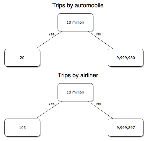
Figure 2. A probability tree to help visualize comparison of deaths (“yes”) by car travel and by airline travel in the United States for the year 2000.
Comparing rates and proportions
Without going into the details, we will do so in Chapter 9 Inferences on Categorical Data, comparing two rates is a chi-square, χ2, contingency table type of problem. More specifically, however, it is a binomial problem (Chapter 3.1, Chapter 6.5); there are two outcomes, death or no death, and we can describe how likely the event is to occur as a proportion. Because the numbers are large, we can use rely on the normal distribution for comparing the two proportions. We’ll explain this more in the next chapters, but for now it may be enough to present the equation for the comparison of two proportions under the assumption of normality, proportion z test.
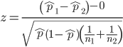
and the null hypothesis (see Chapter 8) tested as that the two proportions are equal. This may be written as
H0 : p1-p2=0
We can assign statistical significance to the differences in events for the two modes of travel under this set of assumptions. Rcmdr has a nice menu-driven system for comparing proportions, but for now I will simply list the R commands.
At the R prompt type each line then submit the command.
total = 100000000
prop.test(c(19700,14),c(total,total)))
And the R output
prop.test(c(19700,14),c(total,total))

    2-sample test for equality of proportions with continuity
    correction

data:  c(19700, 14) out of c(total, total)
X-squared = 19658, df = 1, p-value < 2.2e-16
alternative hypothesis: two.sided
95 percent confidence interval:
 0.0001940984 0.0001996216
sample estimates:
  prop 1   prop 2
1.97e-04 1.40e-07
There’s a bit to unpack here. R is consistent; when it reports results of a statistical test, it typically returns the value of the test statistic (χ2 = 19658), the degrees of freedom for the test (df = 1), and the p-value (< 2.2e-16).
prop.test() were calculated by the Wilson Score method not the Wald method. While both are parametric tests and therefore sensitive to departures from normality (see Chapter 13.3), formulation of Wilson score method makes fewer assumptions (involving approximations of the population proportions) and therefore is considered more accurate.By convention in statistics, if a p-value, where “p” stands for probability, is less than 5%, we would say that our results are statistically significant from the null hypothesis. Looks pretty convincing to me, the difference of 19,700 deaths compared to 14 deaths is clearly different by any criterion and by the results of the statistical test, the p-value is several orders of magnitude smaller than 5%.
Safer to fly. By far, not even close. And similar conclusions would be reached if we compare different years, or averages over many years, or if we used a different way to express the amount of travel (eg, miles/year) by these modes of transportation.
Are you convinced, really? Is it safer to fly?
Let’s try a little statistical reasoning — what assumptions did I make to do these calculations? We recognize immediately that many more people travel by car: that there are way more cars being driven then there are airline planes being flown. The question then is, have we properly adjusted for this difference? Here are a few considerations. My source for the numbers is the NTS 2001 book published by the U.S. Department of Transportation (U.S. Department of Transportation). We are conducting a risk analysis, and the first step is to make sure that we are comparing “apples with apples.” Here are two alternative solutions that at least compare, “Red Delicious” apples with “Macintosh” apples.
Option 1. There are many, many more licensed drivers than there are licensed commercial airline pilots. The standard comparison offered in the background above compared deaths per licensed car driver, but a different metric for air travel, the rate per passenger. This isn’t as bad of a comparison as it may seem — after all, the majority of deaths in car accidents are of the driver themselves. But it isn’t that hard to make the direct comparison — just find out how many commercial pilots there are — a direct comparison with licensed car drivers (stated above as 190,625,023). From the FAA we see that in 2009 there were 125,738 persons with commercial certificates. Since there are only 20 major airline carriers in the United States now (a few more were active in 2000, but we’ll put this aside), the number of licenses is an over estimate of the actual number we want — how many pilots of commercial airlines — but lets use this number for starters — after all, just because a person has a drivers license doesn’t mean they drive or ride in a car.
Number of deaths/yr: Let’s use 2000 data, a typical year prior to 9/11 (and excluding the Covid-19 pandemic). Airlines: 92 deaths; motor vehicles (includes passenger cars, trucks, etc, but not motorcycles): 37,526 deaths (drivers = 25,567; passengers = 10,695; 86 others).
Which mode of travel is riskier? I get a rate a rate of 7.3 X 10⁻⁴ deaths per commercial pilot, or
92125738
compared to a rate for car drivers of 1.97 X 10⁻⁴ deaths.
To summarize what we have so far, I get a result that suggests car travel is almost four times safer
7.3 x 10-41.97 x 10-4→7.31.97 = 3.7
then traveling by commercial airliner. In whole numbers, these results translate to seven deaths for every 10,000 commercial pilots compared to two deaths for every 10,000 licensed car drivers (Fig 3).
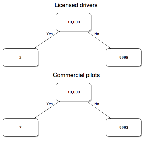
Figure 3. Comparing totals of deaths adjusted by numbers of licensed drivers and by licensed commercial airline pilots in the United States.
R work follows. Enter and submit each command on a separate line in the script window
total = 10000
prop.test(c(2,7),c(total,total))
And the R output
prop.test(c(2,7),c(total,total))

    2-sample test for equality of proportions with continuity
    correction

data:  c(2, 7) out of c(total, total)
X-squared = 1.7786, df = 1, p-value = 0.1823
alternative hypothesis: two.sided
95 percent confidence interval:
 -0.001187816  0.000187816
sample estimates:
prop 1 prop 2
 2e-04  7e-04
What’s happened? The p-value (0.1823) is not less than 5% and so we would conclude under this scenario that there is no difference between the proportions of deaths between the two modes of travel. Let’s keep going.
Option 2. There are many, many more cars on the road then there are airplanes flying commercial passengers. The standard comparison offered in the background information above identified death rates per individual driver, but used a different metric for airline travelers (number of deaths per passenger), which confuses individuals with travelers: what we need is the number of individuals that traveled by airliner, not the total number of passengers (which is many times higher, because of repeat flyers). How can we make a fair comparison for the two modes of travel? Most people never fly whereas most people drive (or ride in a car) frequently in the United States. To me, risk of travel might be better expressed in terms of a per trip rate. I want to know, what are my chances of dying each time I get into my car versus each time I fly on a commercial jet in the United States?
Number of trips/yr. For airlines, I use the number of departures (2000 = 8,951,773). But for cars, we need to decide how to get a similar number. It’s not available directly from the DOT (and would be difficult to get — studies with randomly selected drivers can yield as many as 5 trips per day for licensed drivers). I took the number of licensed drivers and bound the problem — at the low end, let’s say that only 2 trips per week (eg, 50 weeks) are taken by licensed drivers (100 trips); at the upper end, let’s take 2 trips per day per week, or 500 trips/year. Thus, at the low end, we have 1.91 X10¹⁰ trips per year; at the upper end, 9.53 X 10¹⁰ trips per year.
Which mode of travel is riskier? Using the number of deaths/yr listed above in Option 1, I get a rate of 1.03 X 10⁻⁵ deaths/trip for air carriers
928.95 x 10⁶
compared to a rate of 1.97 X 10⁻⁶ deaths/trip for cars (lower bound) or 3.9 X 10⁻⁷ deaths/trip for cars (upper bound). Here’s what the numbers look for in a tree (taking the lower number of trips per year for cars, Fig 4).
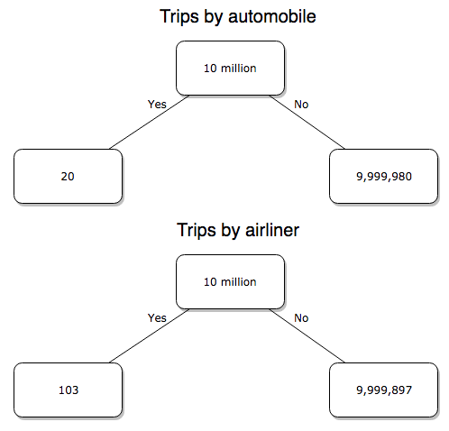
Figure 4. Comparing totals of deaths adjusted by numbers of car trips and by numbers of airline trips in the United States.
R work follow
total = 10000000
prop.test(c(20,103),c(total,total))
And the R output
prop.test(c(20,103),c(total,total))

    2-sample test for equality of proportions with continuity
    correction

data:  c(20, 103) out of c(total, total)
X-squared = 54.667, df = 1, p-value = 1.428e-13
alternative hypothesis: two.sided
95 percent confidence interval:
 -1.057370e-05 -6.026305e-06
sample estimates:
  prop 1   prop 2
2.00e-06 1.03e-05
Now we have another really small p-value (1.428e-13), which suggests a statistically significant difference between the modes of air travel, but the difference in deaths is switched. I now have a result that suggests car travel is much safer than traveling with a commercial airliner! These calculations suggest that you are as much as 26 (upper bounds, five times for lower bounds) times more likely to die from a plane crash then you are behind the wheel. In whole numbers, these results indicate one death for every 100,000 airline flights compared to 1 death for every 500,000 (lower estimate) or 2,500,000 car trips!
Do I have it right and the standard answer is wrong? As Lee Corso used to say on ESPN’s College GameDay program, “Not so fast, my friend!” (Wikipedia). Mark Twain was right to hold the skeptic’s view. Begin by listing the assumptions and by checking the logic of the comparisons (there are still holes in my logic!!). For one, if I am considering my risk of dying by mode of travel, it is far more likely that I will be in a car accident than I will an airline accident, simply because I don’t travel by airline that much. When we consider lifetime risk, we can see why the assertion that it is “safer to fly than drive” is true — we’re far more likely to belong to one of the reference populations involving automobiles (eg, those who drive frequently, for many years) than we are to be among the frequent flyers reference populations.
Questions
1. Review and provide your own examples for
- index
- rate
- ratio
- proportion
3. Like travel safety, we are often confronted by risk comparisons like the following: Which animal is more deadly to humans, dogs or sharks? Between the two, which lead to more hospitalizations in the United States? Work through your assumptions and use results from the International Shark Attack file.
- If a person lives in Nebraska, and never visits the ocean, how does a “shark attack” risk analysis apply? Is it a fair comparison to make between dog attacks and shark attacks? Why or why not.
4. Go to cappex.com/colleges and update institutional (gift) aid offered by Chaminade and HPU. Compare to University of Hawaii-Manoa.
5. Calculate percent increase for
- Annual atmospheric CO2 1980 and 2024.
Quiz Chapter 6.2
Ratios and probabilities
Chapter 6 content
- Introduction
- Some preliminaries
- Ratios and probabilities
- Combinations and permutations
- Types of probability
- Discrete probability distributions
- Continuous distributions
- Normal distribution and the normal deviate (Z)
- Moments
- Chi-square distribution
- t distribution
- F distribution
- References and suggested readings
7.5 – Odds ratio
What are the odds.
We introduced the concept of odds 7.1 — Epidemiology definitions. As a reminder, odds are a way to communicate the chance (likelihood) that a particular event will take place. Odds are calculated as the number of individuals with the event divided by the number of individuals without the event.
Odds ratio definition: is a measure of effect size for the association between two binary (yes/no) variables. It is the ratio of the odds of an event occurring in one group to the odds of the same event happening in another group. The odds ratio (OR) is a way to quantify the strength of association between one condition and another.
Note 1: Effect size — the size of the difference between groups — is discussed further in Chapter 9.2 and Chapter 11.4.
And note, it’s association, not correlation. In statistics, correlation is a specific kind of relationship (linear) among the variables, whereas “association” means there is some relationship between the variables without specifying the shape of the relationship.
How are odds ratios calculated? The probabilities are conditional; recall that conditional probability of some event A, given the occurrence of some other event B.
Let  equal probability of the event occurring (y = Yes) in A,
 equal probability of the event not occurring (n = No) in A,
 equal probability of the event occurring in B, and
 equal probability of the event not occurring in B.
| A | |||
| Yes | No | ||
| B | Yes | |
|
| No | |
|
|
These sum to one: 
The conditional probabilities are
| A | |||
| Yes | No | ||
| B | Yes |  |
 |
| No |  |
 |
|
and finally then, the odds ratio (OR) is
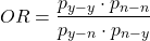
If you have the raw numbers you can calculate the odds ratio directly, too.
| A | |||
| Yes | No | ||
| B | Yes | a | b |
| No | c | d | |
and the odds ratio is then

or, equivalently

Example.
Comparing proportions is a frequent need in court. Gray (2002) provided an example from Title IX of the Education Act of 1972 case Cohen v. Brown University. Under the Act, discrimination based on gender is prohibited. The case concerned participation in collegiate athletics by women. The case data were that of the 5722 undergraduate students, 51% were women, but of the 987 athletes, only 38% were women. A mosaic plot shows graphically these proportions (Fig 1, males in red bars, females in yellow bars).
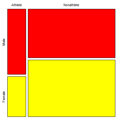
Figure 1. Mosaic plot of athletes to non-athletes in college. Males red, females yellow, data from Gray 2002.
Alternatively, use a Venn diagram to describe the distribution (Fig 2). Circles that overlap show regions of commonality.
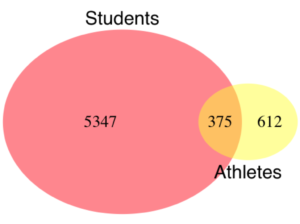
Figure 2. Venn Diagram of athletes to non-athletes in college. Female athletes (n = 375), male athletes (n = 612), data from Gray 2002.
where the orange region

R code for the Venn diagram was
library(VennDiagram)
area1 = 5722
area2 = 987
cross.area = 375
draw.pairwise.venn(area1,area2,cross.area,category=c("Students","Athletes"),
euler.d = TRUE, scaled = TRUE, inverted = FALSE, print.mode = "percent",
fill=c("Red","Yellow"),cex = 1.5, lty="blank", cat.fontfamily = rep("sans", 2),
cat.cex = 1.7, cat.pos = c(0, 180), ext.pos=0)
The question raised before the court was whether these proportions meet the demand of “substantially proportionate.” What exactly the law means by “substantially proportionate” was left to the courts and the lawyers to work out (Gray 2002). Title IX suggests that “substantially proportionate” is a statistical problem and the two sides of the argument must address the question from that perspective.
What is the chance that an undergraduate student was an athlete and female? 38% And the chance that an undergraduate student was an athlete and male? 62% Clearly 38% is not 62%; did the plaintiffs have a case?
Graphs like Figure 1 and Figure 2 help communicate but can’t provide a sense of whether the differences are important. Let’s start by looking at the numbers. Working with the proportions we have the following break down for numbers of students (Table 1) or as proportions (Table 2).
Table 1. Gray’s raw data displayed in a 2 x 2 format.
| Athletes | |||
| Yes | No | ||
| Undergraduates | Male | 612 | 2192 |
| Female | 375 | 2543 | |
Together, the numbers total 5,722.
The Odds Ratio (OR) would be

Or from the proportions (Table 2)
Table 2. Data from Table 1 as proportions.
| Athletes | |||
| Yes | No | ||
| Undergraduates | Male | 0.107 | 0.383 |
| Female | 0.066 | 0.444 | |
adding all of these frequencies together equal 1. Carry out the calculation of odds (Table 3), the conditional probabilities (in bold).
Table 3. Odds calculated from Table 2 inputs.
| Athletes | |||
| Yes | No | ||
| Undergraduates | Male | 0.218
|
0.782
|
| Female | 0.129
|
0.871
|
|
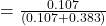
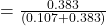
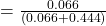
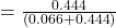
Calculate the odds ratio

Thankfully, whether we use the raw number format or the proportion format, we got the same results!
Odds ratio interpretation.
Because the Odds Ratio (OR) was greater than 1, males students were more likely to be athletes than female students. If there was no difference in proportion of male and female athletes, the odds ratio would be close to one. That is a test of statistical inference (eg, a contingency table), but for now, if one is included in the confidence interval, then this would be evidence that there was no difference between the proportions.
And in R? Simple enough, just create a matrix then apply the Fisher test. which we will discuss further in Chapter 9.5.
title9 <- matrix(c(612, 2192, 375, 2543), nrow=2))
fisher.test(title9)
and results
p-value < 2.2e-16
alternative hypothesis: true odds ratio is not equal to 1
95 percent confidence interval:
1.641245 2.185576
sample estimates:
odds ratio
1.893143
Thankfully, they agree. But note, we now have confidence intervals and a p-value, which we use to conduct inference: were the odds “significantly different from 1?” We would conclude, yes! Between the lower limit (1.64) and the upper limit (2.19), the value “1” was excluded. Moreover, the p-value at 2.2e-16 was much less than the standard type I error cut-off of 5% (see Chapter 8).
Before we leave the interpretation, sometimes a calculated odds-ratio is less than one. If our calculated odds ratio for the Title IX case described in Table 1 was less than 1, (say, the numbers were flipped, Table 4) we then the interpretation would be females were more likely to be athletes on college campus.
Table 4. Table 1 data, but order of entry changed.
| Athletes | |||
| Yes | No | ||
| Undergraduates | Female | 375 | 2543 |
| Male | 612 | 2192 | |
Now, calculating the odds via Fisher exact test, the odds ratio is less than one (0.53):
Fisher's Exact Test for Count Data
p-value < 2.2e-16
alternative hypothesis: true odds ratio is not equal to 1
95 percent confidence interval:
0.4575452 0.6092936
sample estimates:
odds ratio
0.5282222
Note this result is for the same data (Table 1 vs Table 4), just the order by which the groups are specified changed. Of course they are related to each other mathematically, and in a simple way. Note that taking the inverse (reciprocal) odds ratio.

will return the comparison we wanted in the first place — the odds a student athlete was male. As long as you keep track of the comparison, of the groups, it may be easier to communicate results when the reported odds ratio is greater than one.
Relative risk v. odds ratio.
We introduced another way to quantify this association as the Relative Risk (RR) and Absolute Risk Reductions in the previous section. Both can be used to describe the risk of the treatment (exposed) group relative to the control (nonexposed) group. RR is the ratio the treated to control group. OR is the ratio between odds of treated (exposed) and control (nonexposed). What’s the difference? OR is more general — it can be used in situations in which the researcher chooses the number of affected individuals in the groups and, therefore, the base rate or prevalence of the condition in the population is not known or is not representative of the population, whereas RR is appropriate when prevalence is known (this is a general point, but see Schechtman 2002 for a nice discussion).
The odds ratio is related to relative risk, but not over the entire range of possible risk. Odds of an event is simply the number of individuals with the event divided by the number without the event. Odds of an event therefore can range from zero (event cannot occur) to infinity (event must occur). For example, odds of eight (1.89:1) means that nearly two male students were student athletes at Brown University for every one female student.
In contrast, the risk of an event occurring is the number of individuals with the event divided by the total number of people at risk of having that event. Risk is expressed as a percentage (Davies et al 1998). Thus, for our example, odds of 1.89:1 correspond to a risk of 1.89 divided by (1 + 1.89) equals 65%.
To get the relative risk we can use

or 1.7% for our example.
In this example we could use either odds or relative risk; the key distinction is that we knew how many events happened in both groups. If this information is missing for one group (eg, control group of the case-control design), then only the odds ratio would be appropriate.
From cumulative wisdom in the literature (eg, Tamhane et al 2107), if prevalence is less than ten percent, OR ≈ RR. We can relate RR and OR as
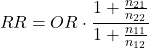
where n11 and n21 are the frequency with the condition for group 1 and group 2, respectively, and n12 and n22 are the frequency without the condition for group 1 and group 2, respectively. For the examples on this page group 1 is the treatment group and group 2 is the control group.
Hazard ratio
The hazard ratio is the ratio of hazard rates. Hazard rates are like the relative risk rates, but are specific to a period of time. Hazard rates come from a technique called Survival Analysis (introduced in Chapter 20.9). Survival analysis can be thought of as following a group of subjects over time until something (the event) happens. By following two groups, perhaps one group exposed to a suspected carcinogen vs. another group matched in other respects except the exposure, at the end of the trial, we’ll have two hazard rates: the rate for the exposed group and the rate for the control group. If there is no difference, then the hazard ratio will be one.
Hazard ratios are more appropriate for clinical trials; relative risk is more appropriate for observational studies.
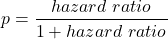
For a hazard ratio, it is often easier to think of it as a probability (between 0 to 1). To translate a hazard ratio to a probability use the following equation
Questions
- Distinguish between odds ratio, relative risk, and hazard ratio.
- Refer to problem 1 introduced in 7.4 – Epidemiology: Relative risk and absolute risk, explained.
Quiz Chapter 7.5
Odds ratio
Chapter 7 contents
7.1 – Epidemiology definitions
Introduction
This subchapter may lack for drama, but let’s start by providing a list of key terms with definitions as you start our introduction to epidemiology. More definitions will follow in the sections as well.
Definitions
Absolute risk: The probability that a specified event will occur in a specified population. See Ch07.4 – Epidemiology: Relative risk and absolute risk, explained.
Absolute risk reduction (ARR): the decrease in risk of an event in an exposed (treatment) group compared to an unexposed (control) group. Also called the risk difference.  , see Contingency table. See Ch07.4 – Epidemiology: Relative risk and absolute risk, explained.
 : Control Event Rate and Experimental Event Rate. In observational studies, transition from “control” and “experimental” to exposure terms. For example, prospective or retrospective cohort studies,
 is Exposed Event Rate and its partner
 , Unexposed Event Rate. Equivalently, you will encounter
 for Incidence in the Exposed and
 forIncidence in the Unexposed. For Case-Control studies, where the direct event (incidence) rates over time are unavailable, then becomes Exposure Rate in Cases — the proportion of people with the condition who were exposed to the risk factor and
 is now Exposure Rate in Controls.
Contingency table, also called cross tabulation or crosstab, is a display of counts of variables in a matrix format. We briefly introduced the contingency table in Chapter 5.1. In epidemiology, rows of contingency table represent treatment or exposure groups, columns represent outcomes.
Table 1. A 2 X 2 contingency table
| Outcome | ||
| Yes | No | |
| Treatment or exposed group | a | b |
| Control or nonexposed group | c | d |
The 2X2 contingency table is referred to frequently in this chapter and again in Chapter 9.
R code
a = 4; b = 46; c = 5; d = 45

Table1 <- matrix(c(a,b,c,d), 2, 2, byrow=TRUE, dimnames = list(c("Treatment", "Control"), c("Yes", "No"))); Table1
R output
          Yes  No
Treatment   4  46
Control     5  45
In statistical classification, a field dedicated to establishing algorithms for correctly identifying and predicting classes of data, eg, correct disease diagnosis or , the 2X2 contingency table is often called a confusion or error matrix (Greene 2003). Machine learning methods are often built on developments from statistical classification findings (Michie et al 1995). We expand on contingency tables in Chapter 7.4 and Chapter 9.2.
Note 1: First discussed in Chapter 5.1, by convention, the standard format for an epidemiological 2×2 contingency table organizes exposure on the rows and disease outcome on the columns as follows:
- Rows (Exposure): The top row represents Exposed / Treatment (Yes), and the bottom row represents Non-exposed / Control (No).
- Columns (Outcome): The left column represents Disease / Case (Yes), and the right column represents No Disease / Control (No). See Chapter 7.
Control event rate (CER): How often an event occurs in the control group.  , see Contingency table.
Diagnosis: identification of the nature of a disease or condition.
Event: From probability theory, an event is a set of one or more outcomes to which a probability is assigned to each outcome.
Experimental event rate (EER): How often an event occurs in the treatment group.  , see Contingency table.
Exposure risk: the potential for harm from contact with or vulnerability to a hazard or risk factor.
Hazard: anything that can cause harm.
Incidence: the number of newly diagnosed individuals in a population having a condition, disease or other characteristic. Compare to prevalence.
Likelihood: In every-day English, the term likelihood and probability mean the same thing — the chance that an event will occur. In statistics, however, probability refers to possible outcomes in the future — a prediction for an event to occur, whereas likelihood is associated with the possible explanation (hypothesis) for the outcome that has already occurred, the past. Put another way, likelihood quantifies how likely is the data we observe, given the hypothesis (cf. excellent discussion by Gallistel 2015)? We will look at likelihood methods in practice in subsequent chapters.
Negative predictive value of a test (NPV), defined as the probability that a negative test result identifies a person who truly does not have the disease. Calculated as the total number of individuals without the disease divided by the total that tested negative. 
Number needed to treat (NNT): the inverse of the absolute risk reduction. 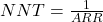 . See Ch07.4 – Epidemiology: Relative risk and absolute risk, explained.
Odds, the ratio (OR) of two probabilities: the probability of getting a one on throwing a dice is  , the probability of not getting a one is
 , therefore the odds of getting a one are 1 to 5.
 . See Ch07.5 – Odds ratio.
Outcome, the single result from a random experiment. For example, result of a single coin toss is “heads.” Results of a birth, the outcome is the child born is a singleton, single birth.
Per capita rate, Latin phrase, for each head, meaning per person.
Positive predictive value of a test (PPV), defined as the probability that a positive test result identifies a person who truly has the disease. Calculated as the total number of individuals with the disease divided by the total that tested positive. 
Posttest probability refers to the probability that the patient has the disease after the results of the test are known.
Pretest probability is the prevalence of the disease, ie, the chance that the a randomly selected person from the population has the disease.
Prevalence: The proportion of individuals in a population having a condition, disease, or characteristic. Compare to incidence.
Probability, defined in Chapter 6.1.
Prognosis, how a disease plays out.
Relative risk: Ratio of the risk of an event among those exposed to the risk factor to the risk among those not exposed to the risk factor. See Ch07.4 – Epidemiology: Relative risk and absolute risk, explained.
Relative risk reduction (RRR): is a measure calculated by dividing the absolute risk reduction by the control event rate. See Ch07.4 – Epidemiology: Relative risk and absolute risk, explained.
Risk: Probability of an event. Risk is not restricted to just bad events, but refers to the uncertainty of a particular event (eg, the risk that a child will be born male seems a melodramatic statement, but it is accurate as far as this definition goes).
Therapy, treatment intended to treat, relieve, or cure a disorder of condition.
Questions
- Compare and contrast ARR and RRR.
- What’s the difference between event, hazard, and risk?
- What’s the difference between incidence and prevalence?
- What’s the difference between diagnosis and prognosis?
- What’s the implication of a NNT greater than 100 in terms of the utility of a proposed therapy or treatment?
Quiz
Quiz Chapter 7.1
Epidemiology definitions
Chapter 7 contents
- Introduction
- Epidemiology definitions
- Epidemiology basics
- Conditional Probability and Evidence Based Medicine
- Epidemiology: Relative risk and absolute risk, explained
- Odds ratio
- Confidence intervals
- References and suggested readings
6.3 – Combinations and permutations
Introduction
In statistical inference, an important foundational skill is to be able to count the possible outcomes of an experiment — the sample space. For example, when drawing on a sample of individuals for study from specific groups (strata) of a population, combinations may be calculated; where it is unwarranted to assume a particular theoretical probability distribution applies, permutation tests create a reference distribution by calculating all possible values of a test statistic under rearrangements of the observed data.
The simplest place to begin with probability is to define an event — an event is an outcome — a “Heads” from a toss of coin, or the chance that the next card dealt is an ace in a game of Blackjack. In these simple cases we can enumerate how likely these events are given a number of chances or trials. For example, if the coin is tossed once, then the coin will either land “Heads” or “Tails” (Fig 1).
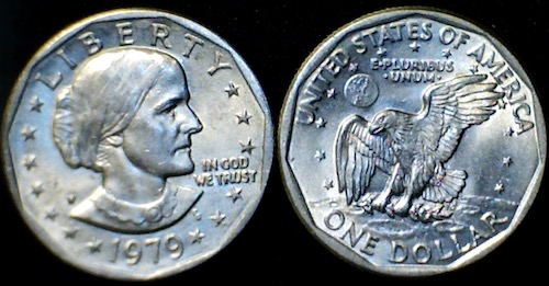
Figure 1. Heads (left) and Tails (right) of a USA Susan B. Anthony dollar.
We can then ask what is the likelihood of ten “Heads” in ten tosses of a fair coin?
And this gets us to some basic rules of probability:
- if successive events are independent, then we multiply the probability
- if events are not independent, then the probability adds
- do we sample without replacement, ie, an object can only be used once?
- do we sample with replacement, ie, an object gets placed “back in the deck” and can be used again and again
Combinations and Permutations
Both combinations and permutations pertain to how samples are selected from a population. Combinations are used if the events or objects of the sample are all of the same kind, whereas for permutations, it is implied that the events or objects are not all of the same kind.
Figure 2. A combination lock
Combinations ignore the order of the events; permutations are ordered combinations. For replacement, the formula for permutations is simply 
In the case of the ten “Heads,” in ten successive trials, the probability is  “ten-times” or
 = 0.0009766 (in R, just type
0.5^10 or (1/2)^10 at the R prompt).
Examples of permutations in biology include,
Given the four nucleotide bases of DNA, adenine (A), cytosine (C), guanine (G), and thymine (T), how many codons are possible?

where the three (3) refers to the codon, three nucleotide genetic code. Codons are trinucleotide sequences of DNA or RNA that correspond to a specific amino acid. For transcription initiation of a protein-coding gene, a key sequence must be present in the promoter region of the gene. In Archaea and Eukaryotes, that sequence is called the TATA box. How often do we expect to find by chance the heptamer (ie, seven bases) TATA box sequence in the human genome?
Note 1: The consensus TATA box sequence, TATAWAW (W can be either Adenine or Thymine, per Standard IUB/IUPAC nucleic acid code). The TATA box is the binding site for transcription factors, particularly the TATA binding protein.

Thus, we would expect at random to find TATA box sequences every 16,384 bases along the genome. For the human genome of 3.3 billion bases then we would expect at random more than 200,000 TATA box consensus sequences.
Another way to put this is to ask how many combinations of ten tosses gets us ten “Heads” then weigh this against all possible outcomes of tossing a coin ten times — how many times do we get zero Heads? Two “Heads”? And so on. This introduces the combinatorial.
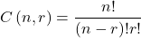
where n is the number of choices (the list of events) and r is how many times you choose or trials. The exclamation point is called the factorial. The factorial instructs you to multiply the number over and over again, “down to one.” For example, if the number is 10, then

In R, just type factorial(10) at the R prompt.
factorial(10)
[1] 3628800
An example
Consider an extrasensory perception, ESP, experiment. We place photocopies of two kinds of cards, “Queen” and “King,” into ten envelopes, one card per envelope (Fig 2). Thus, an envelope either contains a “Queen” or a “King.”

Figure 2. Playing cards with images commemorating 150th anniversary of Charles Darwin’s Origin of Species. (Design John R. C. White, Master of the Worshipful Company of Makers of Playing Cards 2008 to 2009.)
We shuffle the envelopes containing the cards and volunteers guess the contents of the envelopes, one at a time. We score the correct choices after all envelopes had been guessed. (It’s really hard to set these kinds of experiments up to rule out subtle cues and other kinds of experimental error! Diaconis 1978, Pigliucci 2010, pp. 77 – 83.) By chance alone we would expect 50% correct (eg, one way to game the system would have been for the volunteer simply to guess “Queen” every time; since we had placed five “Queen” cards the volunteer would end up being right 50%).
What are the possible combinations?
Let’s start with one correct; the volunteer could be right by guessing the first one correctly, then getting the next nine wrong, or equivalently, the first choice was wrong, but the second was correct followed by eight incorrect choices, and so on.
We need math!
Let n = 10 and r = 1
Using the formula above we have
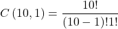
or ten ways to get one out of ten correct. This is the number of combinations without replacement.
In R, we can use the function choose(), included in the base install of R. At the R prompt type
choose(10,1)
and R returns
[1] 10
For permutations, use choose(n,k)*factorial(k).
To get permutations for larger sets, you’ll need to write a function or take advantage of functions written by others and available in packages for R. See gtools package, which contains programming tools for R. There are several packages that can be used to expand capabilities of working with permutations and combinations. For example, install a package and library called combinat and then run the combn() function, together with the dim() function, which will return
dim(combn(10,1))[2]
[1] 10
R explained
In the combn() the “10” is the total number of envelopes and the “1” is how many correct guesses. We also used the dim() function to give us the size of the result. The dim() function returns two numbers, the number of rows and the number of columns — combn() returns a matrix and so dim() saves you the trouble of counting the outcomes — the “[2]” tells R to return the total number of columns in the matrix created by combn(). Here’s the output from combn() , but without the dim() function
combn(10,1)
     [,1] [,2] [,3] [,4] [,5] [,6] [,7] [,8] [,9] [,10]
[1,]    1    2    3    4    5    6    7    8    9    10
in order, we see that there is one case where the success came the first time [1,1], another case where success came on the second try [1,2] and so on.
We can write a simple function to return the combinations
for (many in seq(0, 10, by = 1)){
    print(choose(10, many))
}
an inelegant function, but it works well enough, returning
[1] 1
[1] 10
[1] 45
[1] 120
[1] 210
[1] 252
[1] 210
[1] 120
[1] 45
[1] 10
[1] 1
Note that there’s only one way to get zero correct, only one way to get all ten correct.
For completion, what would be the permutations? Use the permn() function (same combinat library) along with length() function to get the number of permutations
length(permn(10))
[1] 3628800
Continue the example
Back to our ESP problem. If we continue with the formula, how many ways to get two correct? Three correct? And so on, we can show the results in a bar graph (Fig 3).
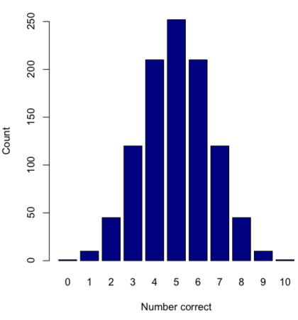
Figure 3. Bar chart of the combinations of correct guesses out of 10 attempts (graph was presented in Chapter 4.1).
The graph in Figure 3 was made in R
Combos <- seq(0,10, by=1)
HowMany <- c(1,10,45,120,210,252,210,120,45,10,1)
barplot(HowMany, names.arg = Combos, xlab = "Number correct", ylab = "Count",col = "darkblue")
If you recall, we had two students score eight out of ten. Is this evidence of “ESP?” It certainly seems pretty good, but how rare is this to score 8 out of 10? The total number of outcomes was

Eight out of ten could be achieved in 45 different ways, so
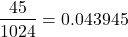
So, eight out of ten is pretty unlikely! Is it evidence for ESP powers in our Biostatistics class? In fact, at the traditional Type I error rate of 5% used in biology and other sciences to evaluate inferences from statistical tests (See Chapter 8), we would say that this observation was statistically significant. Given that this would be an extraordinary claim, this should give you an important clue that statistical significance is not the same thing as evidence for the claim of ESP.
Note 2: This is a good example where frequentist approach may not be the best approach — the Bayesian prior probability for ESP is vanishingly low. See O’Hagan (2006) for a similar ESP problem worked from a Bayesian perspective.
In other words, Is our result biologically significant? Probably not, but I’ll keep my eyes on you, just in case.
Conclusions
Combinations or permutations?
Combinations refers to groups of n things taken k times without repetition. Note that order does not matter, just the combination of things. Permutations, on the other hand, specifically relate the number of ways a particular arrangement can show up.
Questions
- Calculate the combinations, from zero correct to ten correct, from our ESP experiment, ie, confirm the numbers reported in Figure 3.
- Consider our ESP tests based on guessing cards. Let’s say that one subject repeatedly reports correct guesses at a rate greater than expected by chance. Why or why not should we view this as evidence the person may have extrasensory perception?
- Return to our TATA box example. The number of protein-coding genes in the human genome is presently estimated to be 20,620 (NCBI August 2025). Given that each gene has one promoter sequence, what proportion of TATA boxes are not associated with protein-coding genes?
- Assuming a standard 52-card deck, how many possible 5-card poker hands — the set of cards a player holds during a round of play — are there?
Quiz Chapter 6.3
Combinations and permutations
Chapter 6 contents
- Introduction
- Some preliminaries
- Ratios and probabilities
- Combinations and permutations
- Types of probability
- Discrete probability distributions
- Continuous distributions
- Normal distribution and the normal deviate (Z)
- Moments
- Chi-square distribution
- t distribution
- F distribution
- References and suggested readings
6.1 – Some preliminaries
Introduction
OK, you say, I get it: statistics is important, and if I am to go on as a biologist, I should learn statistics. Let’s get on with it, start with the equations and the problems already!
Before we review probability theory and introduce risk analysis I want to spend some time to emphasize that at issue is critical thinking, so please bear with me (Fig 1).
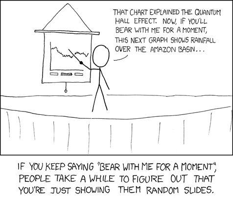
Figure 1. “Slides,” https://xkcd.com/365/.
How likely?
As we start our journey in earnest, we start with the foundations of statistics, probability. Probability in statistics means the chance that a specific outcome will occur. Probability is something we measure, or estimate, or draw from theoretical models, about whether something, a specific outcome from a class of outcomes (events — see Chapter 7.1), will occur. We speak about how likely an outcome is to occur, and this is quantified by the probability. Probabilities are given a value between 0 and 1: at 0% chance, the event will not happen; 100% chance, the event is certain to happen. Remember, probability applies to predicting future events; obviously, when viewed in the past, the event either did (100%), or did not (0%) happen.
If probability is the chance that an outcome will occur, then risk is the probability of a particular outcome occurring over a specified period of time. Related, epidemiologists define exposure risk as the potential for harm (or benefit) from contact with or vulnerability to a hazard (or treatment) or risk factor.
I introduce our discussion of probability through a risk analysis — the process of evaluating the probability and potential impact of health risks to individuals or populations. I like to start this discussion by relaying something I overheard while a number of us were standing on a lava field on the slopes of Kilauea back in November of 1998 (Kilauea erupted with lava flow more or less continually between 1983 and 2018; 5 Jan 2023, started up again).

Figure 2. View of Kamokuna Lava Bench, eruption of Pu`u `O`o, Kilauea, November 1998. Photo by S. Dohm.
In 1998, Volcanoes National Park hadn’t established barricades at the end of Chain of Craters Road, and people were walking to see new lava flows. The night we went, we met a park ranger who pleaded with us that the Park Service believed it was unsafe for us to walk out to see new lava flows because the area, called a lava delta, was unstable. Someone (not in my group), snapped back, “Oh, what are the chances that that will happen?” Of course, the ranger couldn’t quote a chance between zero and 100% for that particular evening. The ranger was saying the risk had increased, based on their subjective, but experienced opinion (see Kinds of probability, below).
As you can see in Figure 2, we went anyway. I have been thinking about her question ever since. We were lucky — some of the same area collapsed two weeks later (SOEST information, eruption about episode 55).
Cool picture though.
While the terms are used interchangeably in everyday language, they have distinct mathematical and statistical definitions. Prospective: You use a known model and its parameters to predict the probability of future data.
Multiple events
Whether or not a newly formed lava delta collapses, that’s a singular or simple event. For cases with more than one one outcome, that’s a multiple event.
I have two coins, a dime and a quarter, in my pocket; when I place the coins on the table, what are the chances that both coins will show heads? A blood sample from a crime scene was typed for two Combined DNA Index System (CODIS) Short Tandem Repeat (STR) loci, THO1 (allele 9.3) and TPOX (allele 8), the same allele types for the defendant. What are the chances of a match, someone other than the defendant has the same genetic profile? In both examples I describe a random process. With randomness, we can predict the probability of each kind of outcome, or series of outcomes, because we know the total possible number of outcomes. If there are just two outcomes, then the probability is equal — 50% that either will occur. If, however, the process is not random, then even if there are just two possible outcomes, the probability can’t be 50% — the outcome depends on some other process than random chance.
What is the chance that two events occur? For two or more independent events we can get the answers by using the product rule.

The two coins are independent, therefore the chance that both are placed heads up is 25% — we would expect to see this combined event one out of every four times. This is an illustration of the counting rule, aka fundamental counting principle: if there are n ways to do one thing (n elements in set A), and m ways to do another thing (m elements in set B), then there are  ways to do both things (combination of elements of A and B sets).
For the DNA profile CODIS problem (cf. Chapter 4, National Research Council 1996), the two alleles are both the most common observed in US Caucasian population at 30.45% and 54.7%, respectively (Moretti et al 2016). Assuming the individual was homozygous at both loci (ie, THO19.3,9.3 and TPOX8,8), then the genotype frequencies (p2) are:


Since THO1 is located on the p arm of chromosome 11, and TPOX is on the p arm of chromosome 2, the two loci are independent and therefore should be in linkage disequilibrium. We can use the product rule to get the probability of the DNA profile for the sample, 2.8%

If two events are not independent, then the product rule cannot be used. For example, CODIS STR D5S818 and CSF1PO are both located on the q arm of chromosome 5 and are therefore linked and not independent (the recombination frequency is about 0.25). The common allele for D5S818 is 11 at 40.84% and for CSF1PO the allele is 12 at 34.16%. Thus the chance that the two most common alleles is not simply the product rule result of 14%, instead we need to view this problem as one of dependent events.
Kinds of probability.
So, how does one go about estimating the likelihood that a particular event, whether it is collapse of a lava delta, or that a person will have a heart attack? The probability of lava delta collapse or of heart attack are examples of empirical probability, as opposed to a theoretical probability. Despite many years of effort, we have no applicable theory that we can apply to say, if a person does this, and that, then a heart attack will happen. But we do have a body of work documenting how often heart attacks occur, and when they occur in association with certain risk factors. Similarly, progress is being made to determine markers of risk of lava field collapse (Di Traglia et al. 2018). Analogously, this is the essential goal of risk analysis in epidemiology. We know of associations between cholesterol and heart attack risk, for example, but we also know that high cholesterol does not raise the probability of the event (heart attack) to 100%. How is this uncertainty part of statistics? Or perhaps you are a molecular scientist in training and have learned about how to assess results of a Western blot where typically the results are scored as “yes” or “no.” How is this relevant to statistics and probability?
A misconception about statistics and statistical thinking
There’s a long history of skepticism of conclusions from health studies, in part because it seems the advice flips. For example,
- Coffee is bad for you (Medical News Today January 2008)
- Coffee is good for you (NBC News July 2018)
- Even light drinking can be harmful to health (Science Daily, January 2022)
- Seven science-backed reasons beer is good for you (NBC News August 2017)
- Meat and cheese may be as bad for you as smoking (Science Daily, March 2014)
- Cheese actually isn’t bad for you (WIRED, February 2021)
The common thread is these studies are assessment of risk: about studies that seem to conclude “only: with statements of probability.
Perhaps you may have heard …? “There are lies and then there is statistics“. The full quote reads as follows:
Figures often beguile me, particularly when I have the arranging of them myself; in which case the remark attributed to Disraeli would often apply with justice and force: “There are three kinds of lies: lies, damned lies and statistics.” – Autobiography of Mark Twain (www.twainquotes.com/Lies.html).
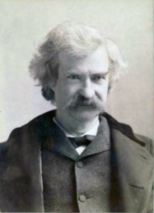
Figure 3. Mark Twain. Image from The Miriam and Ira D. Wallach Division of Art, Prints and Photographs: Photography Collection, The New York Public Library. “Mark Twain in Middle Life” The New York Public Library Digital Collections. 1860 – 1920. https://digitalcollections.nypl.org/items/510d47d9-baec-a3d9-e040-e00a18064a99
Twain attributed the remarks to Benjamin Disraeli, the prime minister of Britain during much of Queen Victoria’s reign, but others have not been able to document this utterance to that effect. Still others believe that the “3-lies” quote belongs to Leonard Courtney, an English mathematician and statistician (1847-1929) (see University of York web site for more).
What is meant by this quote? Tossing aside cynicism — or healthy skepticism of authority one should have, whether that authority is a scientist or a politician(within reason, please!) — what this quote means is that it seems that results of very similar studies are in conflict. To some, this is part of the replication crisis in science (Baker 2016). There’s a perception that one can say just about anything with a number. Partly this is a matter of semantics, but also there is legitimacy to this concern. However, it is not necessarily the case that statistics have been intentionally done to mislead, rather, there is evidence that researchers are not always using proper statistical procedures.
One word, several meanings
We use the term statistics in multiple ways, all correct, but not all equal. For example, a statistic may refer to a number used to describe a population characteristic. From the 2010 U.S. census, we learn that the racial (self-reported) make-up of the U.S. population (then at 303 million) was 72.4% “white” and 12.6% “black” self-reported. In this sense, a statistic is something you calculate as a description. Do you recall the distinction between “statistic” and “statistics” discussed in Chapter 2?
Secondly, two studies essentially about the same topic, yet reaching seemingly different conclusions, may differ in the assumptions employed. It should be obvious that if different assumptions are used, researchers may reach different outcomes.
Finally, how we communicate statistics can be misleading. For example, use of percentages in particular can be confusing, especially in communication of the chance that some event may happen to us (eg, incidence of disease: number of new cases in a specific time period, compared to prevalence of a disease: number of cases of a disease in a specific period of time). On the one hand, percentages seem easy. A percentage is simply a proportion multiplied by 100%, and takes any value between 0% and 100%.
When a product says that it kills 99.99% of all germs on contact, do you feel better? Here’s a cartoon to consider as you think about that statement (Fig 4).
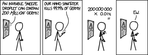
Figure 4. “Hand sanitizer,” https://imgs.xkcd.com/comics/hand_sanitizer.png
Of course numbers cannot be used to justify simultaneously mutually exclusive conclusions, but being able to recognize careless (or deliberate) miscommunication with numbers, well, this needs to be part of your skill set. Here’s a little exercise from transportation safety to ponder as you reflect on the subject of lies and statistics. rather, as you read this next section I ask that you consider
- are the correct statistical descriptors in use?
- what assumptions are being made?
- does the reporting of percentages lead to clear conclusions?
Some concluding thoughts about “lies and statistics”
Statistics is tricky because there are assumptions to be made. And you have to be clear in your thinking.
If the assumptions hold true, then we aren’t lying, and Twain had it wrong.
But if we disagree on the assumptions, then we will necessarily have to disagree on the conclusions drawn from the calculated numbers (the statistics). Risk analysis in particular, but statistics in general, is a tricky business because many assumptions need to be made, and we won’t necessarily have all of the relevant information available to make sure our assumptions are truthful. But it is the assumptions that matter: if we agree with the assumptions that are made, then we have confidence in the conclusions drawn from the statistics.
In a typical statistics course, we would spend a bunch of time on probability. We will here as well, but in the context of risk analysis and in the other contexts, in a less than formal presentation on the subject of probability. For example, in talking about inference, the testing of null hypotheses and estimating the probability that the null hypothesis is correct, I will say things like, “Imagine we repeated the experiment a million times — how many times by chance would we think a correct null hypothesis would none the less be rejected?”
There’s no real substitute for a formal course in probability theory and you should be aware that this foundation is pretty important if you go forward with biostatistics and epidemiology. For now, I will simply refer you to chapters 1, 2 and 3 of a really nice online book on probability from one of the masters, Richard Jeffrey (1926 – 2002; click here to go to Wikipedia). Much of what I will present to you follows from similar discussions.
My aim is to teach you what you need about probability theory by the doing. In the next couple of days we will deal with an aspect of risk analysis, namely a consideration of conditional probability and Baye’s Theorem that will help you evaluate claims such as the one made for airline safety. Risk analysis is tricky, but it is not a subject above and beyond our abilities; by applying some of the rules of statistical reasoning, we can check claims based on statistics. A healthy degree of skepticism is part of becoming a scientist. Do try this at home!
Some examples to consider: what is the relative risk for the following scenarios?
1. Drug testing at the workplace: risk of a worker, who does not use illegal drugs, registering positive (false positives in drug testing);
2. Positive HIV from blood sample from USA male with no associated risks (eg, intravenous drug user), false positives in HIV testing; false positives with mammography;
3. Benefits versus risks of taking a statin drug (drug that reduces serum cholesterol levels) to a person with no history of heart disease.
4. Is it safer to travel by car or by airliner? We’ll break this problem down in the next section.
What we are looking for is the probability of an occurrence of a particular event: that a person who does not use illegal drugs may nonetheless test positive; we are looking for a way to make rational decisions and understanding probability is the foundation.
Questions
- What do you make of the claim (joke) that “There are lies and then there are statistics?”
- Distinguish between empirical and theoretical probability; use examples.
Quiz Chapter 6.1
Some preliminaries
Chapter 6 contents
- Introduction
- Some preliminaries
- Ratios and proportions
- Combinations and permutations
- Types of probability
- Discrete probability distributions
- Continuous distributions
- Normal distribution and the normal deviate (Z)
- Moments
- Chi-square distribution
- t distribution
- F distribution
- References and suggested readings
2.3 – A brief history of (bio)statistics
Foundations of biostatistics: key definitions.
.
Before discussing history and landmark moments in biostatistics, let’s start with basic definitions.
Bioinformatics is loosely defined as a discipline of biology primarily concerned with work involving large data sets (eg, databases), but a bioinformatician would not primarily be a statistician necessarily. Rather, a bioinformatician in addition to foundation in statistical and mathematical training would likely be fluent in at least one programming language and confident in use and design of databases.
Biostatistics, or biometry, then, refers to use of statistics in biology. Biostatistics encompasses application of statistical approaches to design, analyze, and interpret biological data collected through observation of use of experimentation. In turn, there are many broad disciplines or fields of specialty that trained biostatisticians may work.
Chance, the likelihood that a particular event will occur.
Data scientist, a very general label, is a person likely to work on “big data.” Big data may be loosely and inconsistently identified as access to large detailed and unstructured data sets such as visits and behavior within websites of tens of millions of Internet “hits” to a website like Amazon® or Google®. The data scientist would then be involved in extracting meaning from volumes of this data in a process called data mining. In the context of biology web sites like allele frequency aggregator at NCBI, which houses allele frequency information collected on human populations, the 1000 genome project, or any of the databases accessible at National Center for Biotechnology Information would constitute sources of big data for biological researchers.
Epidemiology refers to the statistics of patterns of and risk of disease in populations, particularly of humans and thus, an epidemiologist would also be considered to be a biostatistician. The statistics of epidemiology include all of the materials we will cover in this course, but perhaps if any particular analytical approach characterizes epidemiology, it would be survival analysis (review in Clark et al 2003) — in competition with compartment models to predict spread of communicable disease in populations (Brauer 2017).
Event, an outcome to which a probability is assigned.
Likelihood, the probable chance of occurrence of an event that has already occurred. Likelihood assesses how well a particular model or set of parameters explains observed data.
Probability, the chance that an event will occur in the future, given a known model or set of parameters.
Random or random chance. This is a good place to share a warning about vocabulary; statistics, like most of science, uses familiar words, but with refined and sometimes different meanings than our everyday usage. Consider our everyday use of random: “without definite aim, direction, rule, or method – subjects chosen at random” (Merriam-Webster online dictionary). In statistics, however, random refers to “an assignment of a numerical value to each possible outcome of an event” (Wikipedia, Eagle 2021). Thus, in statistics, random dictates a method of determining how likely a subject is to be included: If  represents the size of the population, then random sampling implies that each individual had
 chance of being selected. Thus, if
 , then each individual has a 1% (
 ) chance of selection. This is quite different from Merriam-Webster’s definition, in which no method is assumed. To a statistician, then, random as used in everyday conversation would imply haphazard sampling or convenience sampling from a population.
Statistics may be defined as the science of collecting, organizing, and interpreting data. Statistics is a branch of applied mathematics. Note that the word statistic is also used, but refers to a calculated quantity like the mean or standard deviation. A little confusing, but the context in which statistics or statistic is appropriate is usually not a major issue.
Note 1. Did you notice how the definitions for chance, likelihood, and probability were rather circular? Of the three, chance is more informal while both likelihood and probability are distinct concepts in statistics.
From dice games to data science: A brief history of statistics.
.
Figure 1. Soldiers playing dice, painting by Michiel Sweerts (1618–1664). Public domain image, https://commons.wikimedia.org/
The concepts of chance and probability, so crucial to statistical reasoning — because it allows us to interpret data when outcomes are inconsistent — were realized rather late in the history of mathematics. While people have been writing about applied and theoretical math for thousands of years, probability as a topic of interest by (Western) scholars seems to date only back to the late 17th century, beginning with letters written between Pierre de Fermat (1601-1665) and Blaise Pascal (1623 – 1662) and the substantial work on probability by Pierre-Simon Laplace (1749-1827). Often, research on probability developed under the watchful eyes of rich patrons more interested in gaming (sensu Fig 1), than to scientific applications. Work on permutations and combinations, essential for an understanding of probability, trace to India prior to Pascal’s work (Raju 2011).
The history of statistics goes back further if you allow for the dual use of the term statistics, both as a descriptor of the act of collecting data and as a systematic approach to the analysis of data. Prior to the 1700s, statistics was used in the sense of collection of data for use by the governments. It is not until the latter part of the 19th century that we see scholarship on statistical analytical techniques. Many of the statistical approaches we teach and use today were developed in the decades between 1880s and the 1930s. Work by Francis Galton (1822-1911), Karl Pearson (1857-1936), RA Fisher (1890-1962), Sewall Wright (1889-1988), Jerzy Neyman (1894-1981), Egon Pearson (1895-1980, Karl Pearson’s son), George EP Box (1919-2013) remains highly influential today.
Development of randomized controlled (clinical) trials, RCT, the “gold standard,” by the 1950s provides the strongest study design to evaluate the effectiveness of clinical or other kinds of interventions. The general features of RCT are (1) comparison among groups, with at least one control group, (2) randomization, and (3) blinding, where treatment options are concealed from the subjects (single-blind) and from those charged to assess the outcomes (double-blind). Sir Austin Bradford Hill (1887-1991) is generally credited with developing the RCT (Collier 2009, Matthews 2016), but we owe RA Fisher for randomization in experimental design. Hill (1965) is also known for Hill’s criteria of causality — nine principles that can be used to establish causal relationship between epidemiological (observational) evidence and disease. Chief among these nine principles are strength of the association (effect size) and consistent association (reproducibility), elements we return to often in our introduction to biostatistics.
Since the 1950s, there has been an explosion of developments in statistics, particularly as related to power of computer. These include use of resampling, simulation, and Monte Carlo methods (Harris 2010). Resampling — the creation of new samples based on a set of observed data — is a key innovation in statistics. Its use led to a number of innovative ways to estimate the precision of an estimate (see Chapter 3.4 and Chapter 19). Monte Carlo methods, or MCM, which involves resampling from a probability distribution, is used to repeat (simulate) an experiment over and over again (Kroese et al 2014). Computers have so influenced statistics that some now define statistics as “…the study of algorithms for data analysis” (p 175, Beran 2003). So much so, the role of computers and coding to process and model data, we now have the discipline of Data Science. For more on the history of statistics, see Anderson (1992), Fienberg (1992), and Freedman 1999; for excellent, conversational books read Salsburg (2002) and McGrayne (2011). For influential women in early development of statisticians, see Anderson (1992).
Numbers and prejudice: A hidden history of statistics.
.
Many statistical methods in use today, including regression and analysis of variance methods, can trace their origins to the late 1800’s and early 1900’s (Kevles 1998). Many of these early statisticians developed statistical methods to, at least in part, further their interests in understanding differences between racial groups of humans. Sir Francis Galton, who developed regression and correlation concepts (the details and extensions of which were the works of Karl Pearson), coined the term Eugenics, the “science” of improving humans through selective breeding. In an editorial, the journal Nature recently published an apology for it’s complicity providing “a platform to [eugenicists] views” (p 875, Nature 2022). Sir RA Fisher is rightfully remembered as the inventor of analysis of variance and maximum likelihood techniques (Rao 1992; Bodmer et al 2021), and perhaps more important, developed the concepts of sampling from populations, degrees of freedom, among other contributions. Moreover, work of Fisher, Wright, and others led to the realization that populations of the same species differed at many locations in the genome, thus completely refuting any notion of “racial purity” (Bodmer et al 2021). However, Fisher was an active promoter of eugenics (Bodmer et al 2021), and an award given by The Society for the Study of Evolution in his honor, the RA Fisher Prize, was renamed in 2020.
Eugenics is still with us (Liscum and Garcia 2022; see also Legacies of Eugenics: An Introduction Los Angeles Review of Books; Veit et al 2021), but the era of “Three generations of imbeciles are enough” (Buck v. Bell), and the forced sterilization eugenic programs of the Nazi (Kelves 1999), were thoroughly discredited on scientific grounds many times (click here for Eugenics Archive website). Do keep in mind that the times were different, and elements of eugenics thinking remains with us (cf discussion in Veil et al 2021 and references therein), it is interesting nevertheless to learn about the murky history of statistics and the objectives of some of the very bright people responsible for many of the statistical analyses we use today (see Stephen J. Gould’s “The Mismeasure of Man“). Several books tackle aspects of scientific racism, including 2017 Is science racist? by Jonathan Marks and 2019 Superior: The return of of race science, by Angela Saini, Cathy O’Neil’s 2017 accessible book Weapons of math destruction: How big data increases inequality and threatens democracy, and a host of articles and books listed at Wikipedia.
Keep in mind also that geneticists and statisticians were instrumental in showing why Eugenics was unscientific, at best. See partial listing in Bodmer et al (2021). Also, see 2021 review by Rebecca Sear, Demography and the rise, apparent fall, and resurgence of eugenics, in Population studies: A journal of demography. While the algorithms of statistics should be unbiased — and we often believe that they are — clearly, humans, and the interpretations of data may be biased (Celiktutan et al 2024). Statistical reasoning absolutely requires considering sources of bias and their impacts on our conclusions.
Landmark epidemiology studies.
.
John Snow (1813-1858) is credited by some as the “Father of Epidemiology”(Ramsay 2006). During a London outbreak — the sudden increase of disease events — of cholera in 1854, Snow conducted work to establish cholera mortality with source and quality of drinking water. At the time, the prevailing explanation for cholera was that it was an airborne infection. Snow’s map of cholera mortality in the Golden Square district of London in relation to a water pump on Broad Street is shown in Fig 2, Snow’s theory of contaminated water was not accepted as an explanation for cholera until after his death.
Original map by John Snow showing the clusters of cholera cases in the London epidemic of 1854, drawn and lithographed by Charles Cheffins.
Figure 2. Original map by John Snow showing the clusters of cholera cases in the London epidemic of 1854, drawn and lithographed by Charles Cheffins. Image Public Domain, from Wikipedia.

Snow’s work and dataset can be viewed and thanks to Paul Lindman and others, the work can be expanded: for example, define areas around pumps by walking distance (Fig 3). The R package is cholera. Figure 2 shows a plot like Snow’s annotated map.cholera.
Figure 3. Plot of Snow’s London using R cholera package. Triangles marked with p1-p13 represent public water pumps. Red dots represent cholera cases.
R code to make the plot was
snowMap()Snow’s ideas about cholera were not accepted in his time and you should recognize that by itself, a cluster map supports both the airborne and waterborne theories. The cholera package contains additional data to help visualize the area, including setting regions by walking distance (Fig 4).
Figure 4. Plot of Snow’s London with walking areas drawn about the 13 water pumps. R cholera package.
R code to make the plot was
plot(neighborhoodWalking(case.set = "expected"), "area.polygons")Epidemiology of cancer.
.
This is an undeveloped section in my book. For now, I’ve listed a number of key landmark studies — a selective and incomplete list — in the history of epidemiology and cancer risk — these would serve well as case studies:
- Tobacco as a carcinogen
- Doll R, Hill AB. Smoking and carcinoma of the lung; preliminary report. Br Med J 1950; 2: 739–748
- Fontham ET, Correa P, Wu-Williams A, Reynolds P, Greenberg RS, Buffler PA, Chen VW, Boyd P, Alterman T, Austin DF, Liff J, Greenberg SD. Lung cancer in non-smoking women: a multicenter case-control study. Cancer Epidemiol Biomarkers Prev 1991;1:35-43
- Diet and cancer risk
- Kolonel LN, Hankin JH, Lee J, Chu SY, Nomura AM, Hinds MW. Nutrient intakes in relation to cancer incidence in Hawaii. Br J Cancer 1981;44:332-339.
- Obesity, exercise, and cancer risk
- Calle EE, Rodriguez C, Walker-Thurmond K, Thun MJ. Overweight, Obesity, and Mortality from Cancer in a Prospectively Studied Cohort of U.S. Adults. N Engl J Med 2003;348:1625-1638.
- Hormones and cancer risk
- Marchbanks PA, McDonald JA, Wilson HG, Folger SG, Mandel MG, Daling JR, Bernstein L, Malone KE, Ursin G, Strom BL, Norman SA, Wingo PA, Burkman RT, Berlin JA, Simon MS, Spirtas R, Weiss LK. Oral contraceptives and the risk of breast cancer. New Engl J Med 2002;346(26):2025-2032.
- Cancer risk and occupations
- absence of cervical cancer but high incidence of breast cancer in nuns (Ramazzini, 1713)
- cancer of the scrotums among chimney sweeps of London (Pott, 1775)
- Silverman DT, Hoover RN, Mason TJ, Swanson GM. Motor exhaust-related occupations and bladder cancer. Cancer Res 1986;46:2113-2116.
Please see review by Greenwald and Dunn (2009).
Questions
- Write up three learning outcomes for this page. Hint: Point your favorite generative AI to this page and ask for help.
- Expand my example of landmark studies (also called pivotal or seminal studies) in epidemiology of cancer to a subject of your own interest. For example, vaccination and communicable diseases like polio.
.
Quiz Chapter 2.3
A history of (bio)statistics
Chapter 2 contents
.
- Introduction
- Why biostatistics?
- Why do we use R Software?
- A brief history of (bio)statistics
- Experimental Design and rise of statistics in medical research
- Scientific method and where statistics fits
- Statistical reasoning
- Chapter 2 – References and suggested reading