2.1 – Why (Bio)Statistics?
- What are the basic elements of biostatistics? .
- Why we require you to take Biostatistics as part of your major?.
- But, I’m pre-med and plan to apply to medical school ….
- With machine learning and AI, why learn biostatistics?.
- In what disciplines are biostatisticians employed?.
- Conclusions.
- Questions.
- Quiz.
- Chapter 2 contents
What are the basic elements of biostatistics?
.
What will you learn from an introductory course on (bio)statistics? Concepts and skills: An understanding (concepts) about the purpose and limits of descriptive statistics, inferential statistics, and statistical modeling for answering questions in biology and how to use elements of R programming (skills) applied to biology-related data sets to accomplish these tasks (see Table 1). Related, you will learn how (skills) to collect and manage data from projects, and why (concepts) statistical analysis can help answer questions, even inform decisions in public health. Thus, assessment in BI-311 of student learning includes both formative and summative assignments, exams, and culminates with a student research project.
Note 1: From time to time in this book I write “(bio)statistics” instead of “biostatistics.” It’s my subtle way of highlighting that whatever argument or statement is attached applies more generally to the statistical discipline, not just biostatistics. However, I’m not particularly consistent with this typology in the book.
What skills are you going to get from all of this? You will get different opinions on the elements of an essential first course in statistics or biostatistics. Certainly the basics are a foundation in probability and a breadth of classical elementary statistical procedures, which will include descriptive statistics, analysis of variance and linear regression, and an introduction to multivariate analysis. In preparation for your course in epidemiology you will also be introduced to risk analysis and survival analysis. However, the primary return for your time, I hope, will be a deeper appreciation for how to think about problems in biology from experimental design and data analysis perspectives. Practical skills you will learn include how to process and clean data for analysis, data visualization, and a foundation in parametric and nonparametric statistical methods.
The data sets described and provided in this course are small, with sample sizes in the tens to thousands (rarely). This framework is consistent with the development of the discipline of (bio)statistics, which originated to help interpret experiments conducted in agriculture, industry, and medical research (see Chapter 2.3). But, as you now know, because of genomics and other data-intensive disciplines, data sets can be very large, much beyond the kinds of data sets used prior to use of the computer in data analysis. However, as we will argue later on this page, learning foundational skills in (bio)statistics with small data sets facilitates working with and gaining insights from larger data sets. For example, we will emphasize during our work this semester how to develop a workflow with small data sets; these same workflows then can be scaled up and would include pipelines — based on tools and techniques developed in the broader discipline of bioinformatics — to large data sets, including use of Artificial Intelligence and machine learning.
Note 2: In data science, a workflow refers to the entire, end-to-end process needed in a project, from data collection, data processing, to descriptive statistics and modeling or inferential statistics, and report writing. A pipeline described elements of a workflow that can be automated.
Why we require you to take (Bio)statistics as part of your major?
.
At Chaminade University we require all biology students to take biostatistics, and we do so with an emphasis on use of data analysis skill development. This requirement aligns our program to national expectations of biology undergraduate education (eg, AAAS, NAS, NIH, NSF). As stated in Bio2010: Transforming Undergraduate Education for Future Research Biologists,
“Biology majors should be adept at using computers to acquire and process data, carry out statistical characterization of the data and perform statistical tests, and graphically display data in a variety of representations (p. 15).”
Learning biostatistics from a course like BI311 — which relies heavily on use of the R programming language and data sets — helps the biology student develop these skills.
In the next pages I will outline a history of statistics (Chapter 2.3), but here I wish to make the point that biostatistics is now considered to be a core skill set for biologists. Biostatistics as a discipline came into its own in the 1930’s, but extensive reliance on statistics in research really dates to more recent times because of the ubiquity of personal computers (Salsburg 2002). Modern biological and biomedical research requires computational and quantitative methods to collect, process, analyze, and interpret large data sets. And yet, even a casual survey of required courses for entry into graduate programs in biology (eg, only recommended for admissions to Marine Biology and Cell and Molecular Biology programs at University of Hawaiʻi – Manoa) will reveal that biostatistics is not required of candidates; so, what gives?
The first point is that programs list only minimum requirements. The second point is that many programs (genomics, ecology, etc) will expect the graduate student to take a year or more of (bio)statistics. The need is so crucial that at Harvard Medical School, all biology graduate students are expected to take a crash-course in computing and statistics to work with data (Stefan et al 2015).
Moreover, while graduate programs are not listing statistics as a requirement, many biology undergraduate curricula now require a course in (bio)statistics to reflect the increasingly data driven modern biology — where the jobs are!
My BI-311 students, I’ll make you a bet — or at least, I’ll make this part of your required homework (see BI311 Workbook)! Even a causal search of a research journal article in a biology discipline of your choosing will prove that there is no doing biology research today without an understanding of statistics.
But, I’m pre-med and plan to apply to medical school …
.
Even a cursory look at the literature will result in finding many authors strongly calling for this kind of preparation for a successful career in medicine (eg, Brieger and Hardin 2012). It’s obvious, but needs stating — you’re applying to medical school to become a doctor — you’ll spend the majority of your adult life as a doctor. Statistical thinking is crucial to answering the daily question: “My patient tested positive for biomarker X, what’s the chance that the patient has disease Y?”
Note 3: Following work done by Biomarkers and Surrogate Endpoint Working Group (Clin. Pharmacol. Ther. 69(3), 89–95 2001), biomarkers are biological characteristics that can be “… objectively measured and evaluated as an indicator of normal biological processes, pathogenic processes, or pharmacological responses to a therapeutic intervention” (Naylor 2003). Compare to biomarkers are “[a] defined characteristic that is measured as an indicator of normal biological processes, pathogenic processes, or responses to an exposure or intervention, including therapeutic interventions” (2016 by FDA-NIH Biomarker Working Group in BEST (Biomarkers, EndpointS, and other Tools) Resource).
If your answer today is, the patient has the disease, then you objectively need this course! Hint: there are four possible outcomes, not two, of a test, see Chapter 7.3 – Conditional Probability and Evidence Based Medicine.
Need more convincing? Take a look at the targets of questions intended to evaluate Skill 4 of the Scientific Inquiry and Reasoning Skills standard of the revised MCAT2015 Exam (p. 107, What’s on the MCAT2015 exam?).
- Using, analyzing, and interpreting data in figures, graphs, and tables.
- Evaluating whether representations make sense for particular scientific observations and data.
- Using measures of central tendency (mean, median, and mode) and measures of dispersion (range, interquartile range, and standard deviation) to describe data.
- Reasoning about random and systematic error.
- Reasoning about statistical significance and uncertainty (eg, interpreting statistical significance levels, interpreting a confidence interval).
- Using data to explain relationships between variables of make predictions.
- Using data to answer research questions and draw conclusions.
- Identifying conclusions that are supported by research results.
- Determining the implications of results for real-world situations.
Before we move on, there’s another justification for learning biostatistics we need to discuss.
With machine learning and AI, why learn biostatistics?
Oh, my goodness. If I was starting over, I would definitely want to pursue expertise in machine learning, ML (Fig 2). Machine learning is about finding patterns in large data sets, and modern biological research may be characterized by the impact of large datasets. The machine learning field, and artificial intelligence, AI, in general, are rapidly evolving, but built on more than 20 years of algorithm and computer discoveries. So why not skip biostatistics and go directly to data science?
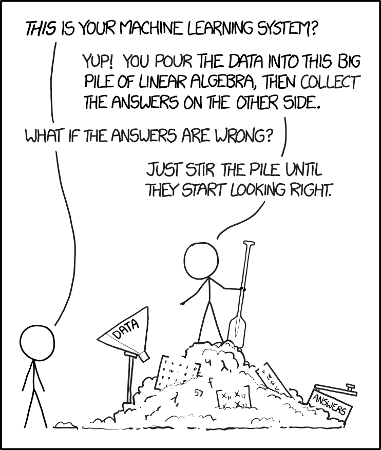
Figure 2. “Machine learning,” https://xkcd.com/1838/.
The parable presented in Figure 2 is about right: Without understanding the statistical foundations behind machine learning algorithms, you’re using tools without really knowing how they work (Lin et al 2025, more generally, see Downey 2024). We have a lot of work ahead of us, but, from time to time, we will exploit the power of AI and ML. For a start, I asked ChatGPT (August 2025), “What statistics is most relevant for ML?”, AI listed responses mapped to “Mike’s Biostatistics Book” are provided in Table 1.
Table 1. AI recommended core statistical topics matched to Mike’s Biostatistics Book
| ChatGPT recommended core statistics topics | Mike's Biostatistics Book |
|---|---|
| Descriptive statistics | Chapter 3 |
| Probability theory | Chapter 6 - 7 |
| Common probability distributions | Chapter 6 |
| Statistical inference | Chapter 8 |
| Estimation and Likelihood | Chapter 3, 6, 17 - 20 |
| Regression analysis | Chapter 17 - 18 |
| Analysis of Variance (ANOVA) | Chapter 12 - 14 |
| Resampling methods | Chapter 19 |
| Dimensionality reduction | Chapter 16, 20 |
| Time series and autocorrelation | Chapter 17 - 18, 20 |
| Optional: Bayesian statistics | Chapter 8 - 9, 18, 20 |
Biostatistics is embedded in bioinformatics and data science, in general. Thus, as implied by Figure 2, a critical step in working with datasets, whether small or large, is to ensure the inputs are valid. This holds across the dat science disciplines. Learning data processing tasks, data cleaning and, more generally, data wrangling are included in our biostatistics course.
Note 4: For larger data sets in the course we will introduce you to rattle, an R package that helps with data processing and data mining with access to simple hypothesis tests (eg, do groups differ?), and pattern detection (eg, correlations and dendrograms). For their required project, students in BI311 may elect to work with the R package targets to build automated data pipelines (eg, calculating growth rates for tomato germination experiments or the essential genes project in Genomics class (BI-308).
In what disciplines are biostatisticians employed?
.
One way to begin this discussion is to think about where statisticians work. The job market includes:
Health Science.
- Drug design, causes of diseases (many “causes” of cancers).
- Health Professional (nurses, physical therapists).
- Type of care and recovery period (importance of a person’s mood on health).
- Exercise regime and recovery from injury.
- Nutrition:- vitamins and health: diet and health.
Ecology & Evolution.
- Causes of changes in population sizes (conservation biology).
- Effects of pollution on organisms and ecosystems.
- Evolution of traits in populations over time.
- Global environmental changes and changes in population sizes or species diversity.
Genetics & Molecular Biology.
- Identifying genes that influence traits (eg, breast cancer, cystic fibrosis).
- Nature vs. nurture (heredity and environment effects on phenotypes).
- Multiple sequence alignment in comparative genomics.
Agriculture.
- Fertilizer effects on plant growth and productivity.
- Compare farming and harvesting methods (eg, organic vs conventional farming).
- Compare plant hybrids for differences in productivity.
Here’s a web site that keeps track of statistics jobs Biostatistics. I would go on to add that experience and competence in statistics would also translate to employment in non-biology fields, eg, business analytics.
Conclusions.
.
Moving forward, we have much to do — you will be exposed to many specific examples of statistical tests, how to calculate estimators, and how to make inferences from experiments. An important goal of this course is for you to be introduced and develop your ability to design experiments. why should you, as biologists and future health care providers, learn biostatistics?
- Develop statistical reasoning skills. Most, if not all graduate students will need to take several courses in statistics.
- Statements about research findings, new and better products, sociological and political issues often depend in large part on some form of statistical analysis.
- By learning a little about experimental design, sampling, and statistical testing, you will be much closer to being able to participate fully in these debates.
- Most, if not all graduate students will need to take several courses in statistics.
- Most, if not all jobs in biology require some training in statistics.
So, there’s really no doing biology without at least some knowledge of statistics. You’re getting a head start!
Questions
- Write up three learning outcomes for this page. Hint: Point your favorite generative AI to this page and ask for help.
- Explore current “biostatistics,” “bioinformatics,” and “data science” job prospects at Indeed.com or other recruiting sites. Search your area/city and also try a wider search.
- Given the rise of AI, now is a great time to explore current thinking about the future and need for biostatistics skills. Write a one paragraph perspective, your “worldview” about pros/cons of developing statistics and data science skill sets.
.
Quiz Chapter 2.1
Why (bio)statistics?
Chapter 2 contents
.
6.1 – Some preliminaries
Introduction
OK, you say, I get it: statistics is important, and if I am to go on as a biologist, I should learn statistics. Let’s get on with it, start with the equations and the problems already!
Before we review probability theory and introduce risk analysis I want to spend some time to emphasize that at issue is critical thinking, so please bear with me (Fig 1).
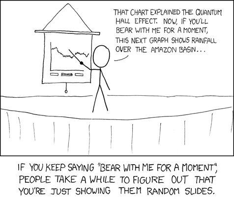
Figure 1. “Slides,” https://xkcd.com/365/.
How likely?
As we start our journey in earnest, we start with the foundations of statistics, probability. Probability in statistics means the chance that a specific outcome will occur. Probability is something we measure, or estimate, or draw from theoretical models, about whether something, a specific outcome from a class of outcomes (events — see Chapter 7.1), will occur. We speak about how likely an outcome is to occur, and this is quantified by the probability. Probabilities are given a value between 0 and 1: at 0% chance, the event will not happen; 100% chance, the event is certain to happen. Remember, probability applies to predicting future events; obviously, when viewed in the past, the event either did (100%), or did not (0%) happen.
If probability is the chance that an outcome will occur, then risk is the probability of a particular outcome occurring over a specified period of time. Related, epidemiologists define exposure risk as the potential for harm (or benefit) from contact with or vulnerability to a hazard (or treatment) or risk factor.
I introduce our discussion of probability through a risk analysis — the process of evaluating the probability and potential impact of health risks to individuals or populations. I like to start this discussion by relaying something I overheard while a number of us were standing on a lava field on the slopes of Kilauea back in November of 1998 (Kilauea erupted with lava flow more or less continually between 1983 and 2018; 5 Jan 2023, started up again).
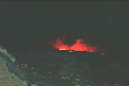
Figure 2. View of Kamokuna Lava Bench, eruption of Pu`u `O`o, Kilauea, November 1998. Photo by S. Dohm.
In 1998, Volcanoes National Park hadn’t established barricades at the end of Chain of Craters Road, and people were walking to see new lava flows. The night we went, we met a park ranger who pleaded with us that the Park Service believed it was unsafe for us to walk out to see new lava flows because the area, called a lava delta, was unstable. Someone (not in my group), snapped back, “Oh, what are the chances that that will happen?” Of course, the ranger couldn’t quote a chance between zero and 100% for that particular evening. The ranger was saying the risk had increased, based on their subjective, but experienced opinion (see Kinds of probability, below).
As you can see in Figure 2, we went anyway. I have been thinking about her question ever since. We were lucky — some of the same area collapsed two weeks later (SOEST information, eruption about episode 55).
Cool picture though.
While the terms are used interchangeably in everyday language, they have distinct mathematical and statistical definitions. Prospective: You use a known model and its parameters to predict the probability of future data.
Multiple events
Whether or not a newly formed lava delta collapses, that’s a singular or simple event. For cases with more than one one outcome, that’s a multiple event.
I have two coins, a dime and a quarter, in my pocket; when I place the coins on the table, what are the chances that both coins will show heads? A blood sample from a crime scene was typed for two Combined DNA Index System (CODIS) Short Tandem Repeat (STR) loci, THO1 (allele 9.3) and TPOX (allele 8), the same allele types for the defendant. What are the chances of a match, someone other than the defendant has the same genetic profile? In both examples I describe a random process. With randomness, we can predict the probability of each kind of outcome, or series of outcomes, because we know the total possible number of outcomes. If there are just two outcomes, then the probability is equal — 50% that either will occur. If, however, the process is not random, then even if there are just two possible outcomes, the probability can’t be 50% — the outcome depends on some other process than random chance.
What is the chance that two events occur? For two or more independent events we can get the answers by using the product rule.

The two coins are independent, therefore the chance that both are placed heads up is 25% — we would expect to see this combined event one out of every four times. This is an illustration of the counting rule, aka fundamental counting principle: if there are n ways to do one thing (n elements in set A), and m ways to do another thing (m elements in set B), then there are  ways to do both things (combination of elements of A and B sets).
For the DNA profile CODIS problem (cf. Chapter 4, National Research Council 1996), the two alleles are both the most common observed in US Caucasian population at 30.45% and 54.7%, respectively (Moretti et al 2016). Assuming the individual was homozygous at both loci (ie, THO19.3,9.3 and TPOX8,8), then the genotype frequencies (p2) are:


Since THO1 is located on the p arm of chromosome 11, and TPOX is on the p arm of chromosome 2, the two loci are independent and therefore should be in linkage disequilibrium. We can use the product rule to get the probability of the DNA profile for the sample, 2.8%

If two events are not independent, then the product rule cannot be used. For example, CODIS STR D5S818 and CSF1PO are both located on the q arm of chromosome 5 and are therefore linked and not independent (the recombination frequency is about 0.25). The common allele for D5S818 is 11 at 40.84% and for CSF1PO the allele is 12 at 34.16%. Thus the chance that the two most common alleles is not simply the product rule result of 14%, instead we need to view this problem as one of dependent events.
Kinds of probability.
So, how does one go about estimating the likelihood that a particular event, whether it is collapse of a lava delta, or that a person will have a heart attack? The probability of lava delta collapse or of heart attack are examples of empirical probability, as opposed to a theoretical probability. Despite many years of effort, we have no applicable theory that we can apply to say, if a person does this, and that, then a heart attack will happen. But we do have a body of work documenting how often heart attacks occur, and when they occur in association with certain risk factors. Similarly, progress is being made to determine markers of risk of lava field collapse (Di Traglia et al. 2018). Analogously, this is the essential goal of risk analysis in epidemiology. We know of associations between cholesterol and heart attack risk, for example, but we also know that high cholesterol does not raise the probability of the event (heart attack) to 100%. How is this uncertainty part of statistics? Or perhaps you are a molecular scientist in training and have learned about how to assess results of a Western blot where typically the results are scored as “yes” or “no.” How is this relevant to statistics and probability?
A misconception about statistics and statistical thinking
There’s a long history of skepticism of conclusions from health studies, in part because it seems the advice flips. For example,
- Coffee is bad for you (Medical News Today January 2008)
- Coffee is good for you (NBC News July 2018)
- Even light drinking can be harmful to health (Science Daily, January 2022)
- Seven science-backed reasons beer is good for you (NBC News August 2017)
- Meat and cheese may be as bad for you as smoking (Science Daily, March 2014)
- Cheese actually isn’t bad for you (WIRED, February 2021)
The common thread is these studies are assessment of risk: about studies that seem to conclude “only: with statements of probability.
Perhaps you may have heard …? “There are lies and then there is statistics“. The full quote reads as follows:
Figures often beguile me, particularly when I have the arranging of them myself; in which case the remark attributed to Disraeli would often apply with justice and force: “There are three kinds of lies: lies, damned lies and statistics.” – Autobiography of Mark Twain (www.twainquotes.com/Lies.html).
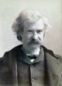
Figure 3. Mark Twain. Image from The Miriam and Ira D. Wallach Division of Art, Prints and Photographs: Photography Collection, The New York Public Library. “Mark Twain in Middle Life” The New York Public Library Digital Collections. 1860 – 1920. https://digitalcollections.nypl.org/items/510d47d9-baec-a3d9-e040-e00a18064a99
Twain attributed the remarks to Benjamin Disraeli, the prime minister of Britain during much of Queen Victoria’s reign, but others have not been able to document this utterance to that effect. Still others believe that the “3-lies” quote belongs to Leonard Courtney, an English mathematician and statistician (1847-1929) (see University of York web site for more).
What is meant by this quote? Tossing aside cynicism — or healthy skepticism of authority one should have, whether that authority is a scientist or a politician(within reason, please!) — what this quote means is that it seems that results of very similar studies are in conflict. To some, this is part of the replication crisis in science (Baker 2016). There’s a perception that one can say just about anything with a number. Partly this is a matter of semantics, but also there is legitimacy to this concern. However, it is not necessarily the case that statistics have been intentionally done to mislead, rather, there is evidence that researchers are not always using proper statistical procedures.
One word, several meanings
We use the term statistics in multiple ways, all correct, but not all equal. For example, a statistic may refer to a number used to describe a population characteristic. From the 2010 U.S. census, we learn that the racial (self-reported) make-up of the U.S. population (then at 303 million) was 72.4% “white” and 12.6% “black” self-reported. In this sense, a statistic is something you calculate as a description. Do you recall the distinction between “statistic” and “statistics” discussed in Chapter 2?
Secondly, two studies essentially about the same topic, yet reaching seemingly different conclusions, may differ in the assumptions employed. It should be obvious that if different assumptions are used, researchers may reach different outcomes.
Finally, how we communicate statistics can be misleading. For example, use of percentages in particular can be confusing, especially in communication of the chance that some event may happen to us (eg, incidence of disease: number of new cases in a specific time period, compared to prevalence of a disease: number of cases of a disease in a specific period of time). On the one hand, percentages seem easy. A percentage is simply a proportion multiplied by 100%, and takes any value between 0% and 100%.
When a product says that it kills 99.99% of all germs on contact, do you feel better? Here’s a cartoon to consider as you think about that statement (Fig 4).
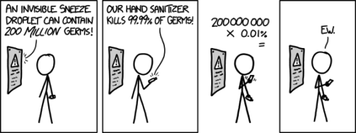
Figure 4. “Hand sanitizer,” https://imgs.xkcd.com/comics/hand_sanitizer.png
Of course numbers cannot be used to justify simultaneously mutually exclusive conclusions, but being able to recognize careless (or deliberate) miscommunication with numbers, well, this needs to be part of your skill set. Here’s a little exercise from transportation safety to ponder as you reflect on the subject of lies and statistics. rather, as you read this next section I ask that you consider
- are the correct statistical descriptors in use?
- what assumptions are being made?
- does the reporting of percentages lead to clear conclusions?
Some concluding thoughts about “lies and statistics”
Statistics is tricky because there are assumptions to be made. And you have to be clear in your thinking.
If the assumptions hold true, then we aren’t lying, and Twain had it wrong.
But if we disagree on the assumptions, then we will necessarily have to disagree on the conclusions drawn from the calculated numbers (the statistics). Risk analysis in particular, but statistics in general, is a tricky business because many assumptions need to be made, and we won’t necessarily have all of the relevant information available to make sure our assumptions are truthful. But it is the assumptions that matter: if we agree with the assumptions that are made, then we have confidence in the conclusions drawn from the statistics.
In a typical statistics course, we would spend a bunch of time on probability. We will here as well, but in the context of risk analysis and in the other contexts, in a less than formal presentation on the subject of probability. For example, in talking about inference, the testing of null hypotheses and estimating the probability that the null hypothesis is correct, I will say things like, “Imagine we repeated the experiment a million times — how many times by chance would we think a correct null hypothesis would none the less be rejected?”
There’s no real substitute for a formal course in probability theory and you should be aware that this foundation is pretty important if you go forward with biostatistics and epidemiology. For now, I will simply refer you to chapters 1, 2 and 3 of a really nice online book on probability from one of the masters, Richard Jeffrey (1926 – 2002; click here to go to Wikipedia). Much of what I will present to you follows from similar discussions.
My aim is to teach you what you need about probability theory by the doing. In the next couple of days we will deal with an aspect of risk analysis, namely a consideration of conditional probability and Baye’s Theorem that will help you evaluate claims such as the one made for airline safety. Risk analysis is tricky, but it is not a subject above and beyond our abilities; by applying some of the rules of statistical reasoning, we can check claims based on statistics. A healthy degree of skepticism is part of becoming a scientist. Do try this at home!
Some examples to consider: what is the relative risk for the following scenarios?
1. Drug testing at the workplace: risk of a worker, who does not use illegal drugs, registering positive (false positives in drug testing);
2. Positive HIV from blood sample from USA male with no associated risks (eg, intravenous drug user), false positives in HIV testing; false positives with mammography;
3. Benefits versus risks of taking a statin drug (drug that reduces serum cholesterol levels) to a person with no history of heart disease.
4. Is it safer to travel by car or by airliner? We’ll break this problem down in the next section.
What we are looking for is the probability of an occurrence of a particular event: that a person who does not use illegal drugs may nonetheless test positive; we are looking for a way to make rational decisions and understanding probability is the foundation.
Questions
- What do you make of the claim (joke) that “There are lies and then there are statistics?”
- Distinguish between empirical and theoretical probability; use examples.
Quiz Chapter 6.1
Some preliminaries
Chapter 6 contents
- Introduction
- Some preliminaries
- Ratios and proportions
- Combinations and permutations
- Types of probability
- Discrete probability distributions
- Continuous distributions
- Normal distribution and the normal deviate (Z)
- Moments
- Chi-square distribution
- t distribution
- F distribution
- References and suggested readings
7 – Probability, Risk Analysis
Introduction
The public health applications of epidemiology, the branch of medicine concerned with identifying patterns and potential causes of disease and health in populations, were every day in the news during the Covid-19 pandemic. From contact tracing to reproductive rate of the SARS-Cov-2 virus to numbers of hospital beds and nurses available in ICU units across the country, to the discussions and debates over how the virus is spread, no doubt you have learned much about the critical role epidemiology continues to play.
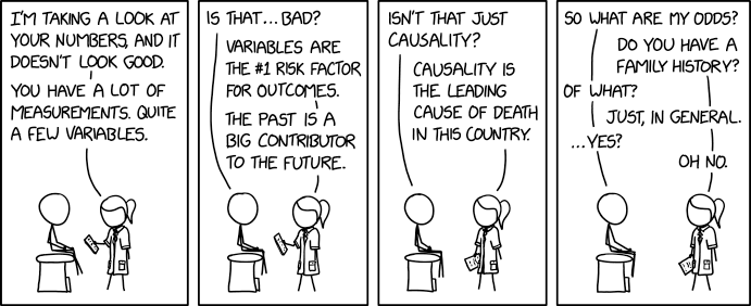
Figure 1. “Health data,” https://xkcd.com/2620/.
This chapter is about probability and introduced you to risk analysis (Fig 1), used to “… characterize the nature and magnitude of risks to human health for various populations…“, a foundational topic in biostatistics and epidemiology. The epiR package will be introduced and code examples provided for descriptive epidemiology and again for statistical inference (Chapter 9).
Homework to go with this topic
Homework 4: Risk in Mike’s Workbook for Biostatistics.
Quizzes in this chapter
A total of 51 questions among the several subchapters, a mix of true or false and multiple choice question format.
Chapter 7 contents
- Introduction
- Epidemiology definitions
- Epidemiology basics
- Conditional Probability and Evidence Based Medicine
- Epidemiology: Relative risk and absolute risk, explained
- Odds ratio
- Confidence intervals
- References and suggested readings
2.3 – A brief history of (bio)statistics
Foundations of biostatistics: key definitions.
.
Before discussing history and landmark moments in biostatistics, let’s start with basic definitions.
Bioinformatics is loosely defined as a discipline of biology primarily concerned with work involving large data sets (eg, databases), but a bioinformatician would not primarily be a statistician necessarily. Rather, a bioinformatician in addition to foundation in statistical and mathematical training would likely be fluent in at least one programming language and confident in use and design of databases.
Biostatistics, or biometry, then, refers to use of statistics in biology. Biostatistics encompasses application of statistical approaches to design, analyze, and interpret biological data collected through observation of use of experimentation. In turn, there are many broad disciplines or fields of specialty that trained biostatisticians may work.
Chance, the likelihood that a particular event will occur.
Data scientist, a very general label, is a person likely to work on “big data.” Big data may be loosely and inconsistently identified as access to large detailed and unstructured data sets such as visits and behavior within websites of tens of millions of Internet “hits” to a website like Amazon® or Google®. The data scientist would then be involved in extracting meaning from volumes of this data in a process called data mining. In the context of biology web sites like allele frequency aggregator at NCBI, which houses allele frequency information collected on human populations, the 1000 genome project, or any of the databases accessible at National Center for Biotechnology Information would constitute sources of big data for biological researchers.
Epidemiology refers to the statistics of patterns of and risk of disease in populations, particularly of humans and thus, an epidemiologist would also be considered to be a biostatistician. The statistics of epidemiology include all of the materials we will cover in this course, but perhaps if any particular analytical approach characterizes epidemiology, it would be survival analysis (review in Clark et al 2003) — in competition with compartment models to predict spread of communicable disease in populations (Brauer 2017).
Event, an outcome to which a probability is assigned.
Likelihood, the probable chance of occurrence of an event that has already occurred. Likelihood assesses how well a particular model or set of parameters explains observed data.
Probability, the chance that an event will occur in the future, given a known model or set of parameters.
Random or random chance. This is a good place to share a warning about vocabulary; statistics, like most of science, uses familiar words, but with refined and sometimes different meanings than our everyday usage. Consider our everyday use of random: “without definite aim, direction, rule, or method – subjects chosen at random” (Merriam-Webster online dictionary). In statistics, however, random refers to “an assignment of a numerical value to each possible outcome of an event” (Wikipedia, Eagle 2021). Thus, in statistics, random dictates a method of determining how likely a subject is to be included: If  represents the size of the population, then random sampling implies that each individual had
 chance of being selected. Thus, if
 , then each individual has a 1% (
 ) chance of selection. This is quite different from Merriam-Webster’s definition, in which no method is assumed. To a statistician, then, random as used in everyday conversation would imply haphazard sampling or convenience sampling from a population.
Statistics may be defined as the science of collecting, organizing, and interpreting data. Statistics is a branch of applied mathematics. Note that the word statistic is also used, but refers to a calculated quantity like the mean or standard deviation. A little confusing, but the context in which statistics or statistic is appropriate is usually not a major issue.
Note 1. Did you notice how the definitions for chance, likelihood, and probability were rather circular? Of the three, chance is more informal while both likelihood and probability are distinct concepts in statistics.
From dice games to data science: A brief history of statistics.
.
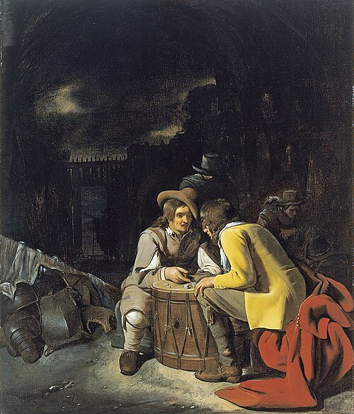
Figure 1. Soldiers playing dice, painting by Michiel Sweerts (1618–1664). Public domain image, https://commons.wikimedia.org/
The concepts of chance and probability, so crucial to statistical reasoning — because it allows us to interpret data when outcomes are inconsistent — were realized rather late in the history of mathematics. While people have been writing about applied and theoretical math for thousands of years, probability as a topic of interest by (Western) scholars seems to date only back to the late 17th century, beginning with letters written between Pierre de Fermat (1601-1665) and Blaise Pascal (1623 – 1662) and the substantial work on probability by Pierre-Simon Laplace (1749-1827). Often, research on probability developed under the watchful eyes of rich patrons more interested in gaming (sensu Fig 1), than to scientific applications. Work on permutations and combinations, essential for an understanding of probability, trace to India prior to Pascal’s work (Raju 2011).
The history of statistics goes back further if you allow for the dual use of the term statistics, both as a descriptor of the act of collecting data and as a systematic approach to the analysis of data. Prior to the 1700s, statistics was used in the sense of collection of data for use by the governments. It is not until the latter part of the 19th century that we see scholarship on statistical analytical techniques. Many of the statistical approaches we teach and use today were developed in the decades between 1880s and the 1930s. Work by Francis Galton (1822-1911), Karl Pearson (1857-1936), RA Fisher (1890-1962), Sewall Wright (1889-1988), Jerzy Neyman (1894-1981), Egon Pearson (1895-1980, Karl Pearson’s son), George EP Box (1919-2013) remains highly influential today.
Development of randomized controlled (clinical) trials, RCT, the “gold standard,” by the 1950s provides the strongest study design to evaluate the effectiveness of clinical or other kinds of interventions. The general features of RCT are (1) comparison among groups, with at least one control group, (2) randomization, and (3) blinding, where treatment options are concealed from the subjects (single-blind) and from those charged to assess the outcomes (double-blind). Sir Austin Bradford Hill (1887-1991) is generally credited with developing the RCT (Collier 2009, Matthews 2016), but we owe RA Fisher for randomization in experimental design. Hill (1965) is also known for Hill’s criteria of causality — nine principles that can be used to establish causal relationship between epidemiological (observational) evidence and disease. Chief among these nine principles are strength of the association (effect size) and consistent association (reproducibility), elements we return to often in our introduction to biostatistics.
Since the 1950s, there has been an explosion of developments in statistics, particularly as related to power of computer. These include use of resampling, simulation, and Monte Carlo methods (Harris 2010). Resampling — the creation of new samples based on a set of observed data — is a key innovation in statistics. Its use led to a number of innovative ways to estimate the precision of an estimate (see Chapter 3.4 and Chapter 19). Monte Carlo methods, or MCM, which involves resampling from a probability distribution, is used to repeat (simulate) an experiment over and over again (Kroese et al 2014). Computers have so influenced statistics that some now define statistics as “…the study of algorithms for data analysis” (p 175, Beran 2003). So much so, the role of computers and coding to process and model data, we now have the discipline of Data Science. For more on the history of statistics, see Anderson (1992), Fienberg (1992), and Freedman 1999; for excellent, conversational books read Salsburg (2002) and McGrayne (2011). For influential women in early development of statisticians, see Anderson (1992).
Numbers and prejudice: A hidden history of statistics.
.
Many statistical methods in use today, including regression and analysis of variance methods, can trace their origins to the late 1800’s and early 1900’s (Kevles 1998). Many of these early statisticians developed statistical methods to, at least in part, further their interests in understanding differences between racial groups of humans. Sir Francis Galton, who developed regression and correlation concepts (the details and extensions of which were the works of Karl Pearson), coined the term Eugenics, the “science” of improving humans through selective breeding. In an editorial, the journal Nature recently published an apology for it’s complicity providing “a platform to [eugenicists] views” (p 875, Nature 2022). Sir RA Fisher is rightfully remembered as the inventor of analysis of variance and maximum likelihood techniques (Rao 1992; Bodmer et al 2021), and perhaps more important, developed the concepts of sampling from populations, degrees of freedom, among other contributions. Moreover, work of Fisher, Wright, and others led to the realization that populations of the same species differed at many locations in the genome, thus completely refuting any notion of “racial purity” (Bodmer et al 2021). However, Fisher was an active promoter of eugenics (Bodmer et al 2021), and an award given by The Society for the Study of Evolution in his honor, the RA Fisher Prize, was renamed in 2020.
Eugenics is still with us (Liscum and Garcia 2022; see also Legacies of Eugenics: An Introduction Los Angeles Review of Books; Veit et al 2021), but the era of “Three generations of imbeciles are enough” (Buck v. Bell), and the forced sterilization eugenic programs of the Nazi (Kelves 1999), were thoroughly discredited on scientific grounds many times (click here for Eugenics Archive website). Do keep in mind that the times were different, and elements of eugenics thinking remains with us (cf discussion in Veil et al 2021 and references therein), it is interesting nevertheless to learn about the murky history of statistics and the objectives of some of the very bright people responsible for many of the statistical analyses we use today (see Stephen J. Gould’s “The Mismeasure of Man“). Several books tackle aspects of scientific racism, including 2017 Is science racist? by Jonathan Marks and 2019 Superior: The return of of race science, by Angela Saini, Cathy O’Neil’s 2017 accessible book Weapons of math destruction: How big data increases inequality and threatens democracy, and a host of articles and books listed at Wikipedia.
Keep in mind also that geneticists and statisticians were instrumental in showing why Eugenics was unscientific, at best. See partial listing in Bodmer et al (2021). Also, see 2021 review by Rebecca Sear, Demography and the rise, apparent fall, and resurgence of eugenics, in Population studies: A journal of demography. While the algorithms of statistics should be unbiased — and we often believe that they are — clearly, humans, and the interpretations of data may be biased (Celiktutan et al 2024). Statistical reasoning absolutely requires considering sources of bias and their impacts on our conclusions.
Landmark epidemiology studies.
.
John Snow (1813-1858) is credited by some as the “Father of Epidemiology”(Ramsay 2006). During a London outbreak — the sudden increase of disease events — of cholera in 1854, Snow conducted work to establish cholera mortality with source and quality of drinking water. At the time, the prevailing explanation for cholera was that it was an airborne infection. Snow’s map of cholera mortality in the Golden Square district of London in relation to a water pump on Broad Street is shown in Fig 2, Snow’s theory of contaminated water was not accepted as an explanation for cholera until after his death.
Original map by John Snow showing the clusters of cholera cases in the London epidemic of 1854, drawn and lithographed by Charles Cheffins.
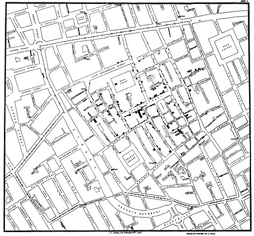
Figure 2. Original map by John Snow showing the clusters of cholera cases in the London epidemic of 1854, drawn and lithographed by Charles Cheffins. Image Public Domain, from Wikipedia.

Snow’s work and dataset can be viewed and thanks to Paul Lindman and others, the work can be expanded: for example, define areas around pumps by walking distance (Fig 3). The R package is cholera. Figure 2 shows a plot like Snow’s annotated map.cholera.
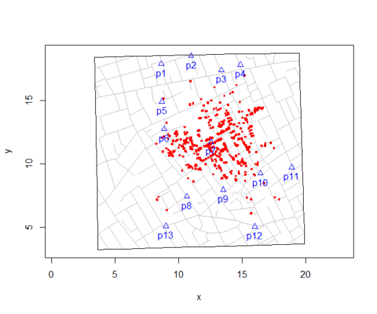
Figure 3. Plot of Snow’s London using R cholera package. Triangles marked with p1-p13 represent public water pumps. Red dots represent cholera cases.
R code to make the plot was
snowMap()Snow’s ideas about cholera were not accepted in his time and you should recognize that by itself, a cluster map supports both the airborne and waterborne theories. The cholera package contains additional data to help visualize the area, including setting regions by walking distance (Fig 4).
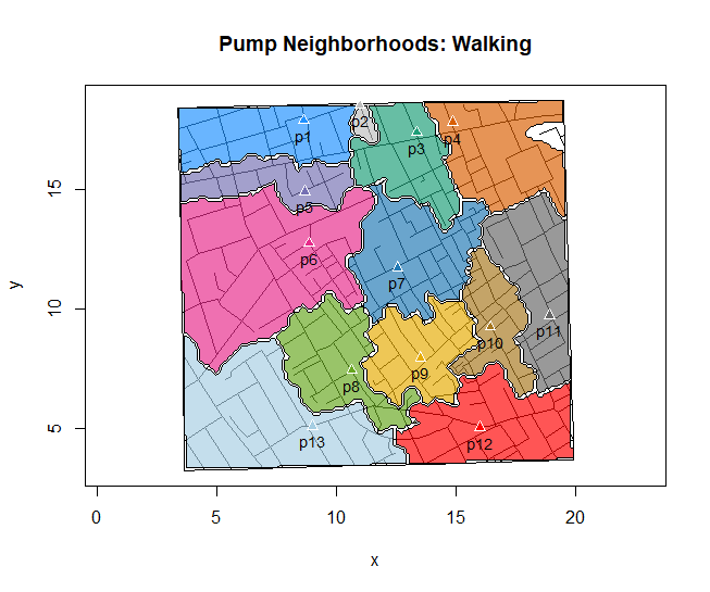
Figure 4. Plot of Snow’s London with walking areas drawn about the 13 water pumps. R cholera package.
R code to make the plot was
plot(neighborhoodWalking(case.set = "expected"), "area.polygons")Epidemiology of cancer.
.
This is an undeveloped section in my book. For now, I’ve listed a number of key landmark studies — a selective and incomplete list — in the history of epidemiology and cancer risk — these would serve well as case studies:
- Tobacco as a carcinogen
- Doll R, Hill AB. Smoking and carcinoma of the lung; preliminary report. Br Med J 1950; 2: 739–748
- Fontham ET, Correa P, Wu-Williams A, Reynolds P, Greenberg RS, Buffler PA, Chen VW, Boyd P, Alterman T, Austin DF, Liff J, Greenberg SD. Lung cancer in non-smoking women: a multicenter case-control study. Cancer Epidemiol Biomarkers Prev 1991;1:35-43
- Diet and cancer risk
- Kolonel LN, Hankin JH, Lee J, Chu SY, Nomura AM, Hinds MW. Nutrient intakes in relation to cancer incidence in Hawaii. Br J Cancer 1981;44:332-339.
- Obesity, exercise, and cancer risk
- Calle EE, Rodriguez C, Walker-Thurmond K, Thun MJ. Overweight, Obesity, and Mortality from Cancer in a Prospectively Studied Cohort of U.S. Adults. N Engl J Med 2003;348:1625-1638.
- Hormones and cancer risk
- Marchbanks PA, McDonald JA, Wilson HG, Folger SG, Mandel MG, Daling JR, Bernstein L, Malone KE, Ursin G, Strom BL, Norman SA, Wingo PA, Burkman RT, Berlin JA, Simon MS, Spirtas R, Weiss LK. Oral contraceptives and the risk of breast cancer. New Engl J Med 2002;346(26):2025-2032.
- Cancer risk and occupations
- absence of cervical cancer but high incidence of breast cancer in nuns (Ramazzini, 1713)
- cancer of the scrotums among chimney sweeps of London (Pott, 1775)
- Silverman DT, Hoover RN, Mason TJ, Swanson GM. Motor exhaust-related occupations and bladder cancer. Cancer Res 1986;46:2113-2116.
Please see review by Greenwald and Dunn (2009).
Questions
- Write up three learning outcomes for this page. Hint: Point your favorite generative AI to this page and ask for help.
- Expand my example of landmark studies (also called pivotal or seminal studies) in epidemiology of cancer to a subject of your own interest. For example, vaccination and communicable diseases like polio.
.
Quiz Chapter 2.3
A history of (bio)statistics
Chapter 2 contents
.
- Introduction
- Why biostatistics?
- Why do we use R Software?
- A brief history of (bio)statistics
- Experimental Design and rise of statistics in medical research
- Scientific method and where statistics fits
- Statistical reasoning
- Chapter 2 – References and suggested reading