20.6 – Dimensional analysis, clustering methods
Introduction
This chapter is just a sampling of the many techniques for “reducing the dimensions” of a data set that contains many variables, aka high-dimensional space, without eliminating the information contained among the many variables. The logic is similar to our discussions about model building — we may seek simple models at least in part so that we can see the big picture, not just each tree in an unhealthy forest.
Approaches can be categorized as feature extraction — a processing step to identify key characteristics contained in the larger data set into fewer, now transformed variables — or feature selection — the selection of a subset of the variables from among the full list which, presumably, contain redundant information. Principal Component Analysis is an example of feature extraction approaches. From this perspective, stepwise regression, discussed in Ch18.5, is an example of a feature selection approach. Clustering methods, however, groups objects based on existing features but does not create new features.
Dimensional analysis and clustering are complementary tools for exploring complex data (Ding and He 2004). Clustering methods use features — or their reduced representations — to group similar objects based on shared patterns. Dimensional analysis and clustering methods, presented together, show how we can first simplify biological complexity and then uncover natural groupings within it, whether we are analyzing candies by color and size or cancerous cells from normal cells by gene expression.
Principal component analysis
High dimensional data are reduced by linear transformation to sets of new vectors or coordinates. Each subsequent vector is orthogonal to the one proceeding it. By orthogonal we mean that variables are uncorrelated, completely independent of each other.
For example, consider body weight and height. Tall people tend to be heavier than shorter people, suggestive of the well-known correlation between the two — body weight and height are not orthogonal. For model building, one can’t simply include both as predictors (multicollinearity). Instead, we use PCA to transform body weight and height into a set of orthogonal variables called Principal Components. The first principal component, PC1, contains the largest amount of variation shared along the first linear adjustment, the second component, PC2, contains the next largest amount of variation, and so on. The result? Because PC2 is orthogonal to PC1, it contains completely different information — the weight that is not explained by height, or residuals.
We demonstrate utility of PCA with Bumpus data from MorphoFun/psa, variable names changed.
First, we plot (Fig 1) and add whether or not the individuals survived (TRUE) or not (FALSE). Figure 1 shows substantial overlap — there’s no distinct separation between the two groups — but survival group (blue) appears to be more concentrated in the lower-left to middle area of the plot. The non survival group (red) extends to higher masses and lengths, with several data points falling outside the main cluster and its corresponding ellipse.
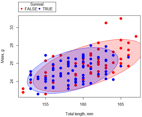
Figure 1. Scatterplot English swallow mass (g) by total length (mm) by survival following winter storm
R code for Figure 1 graph.
car::scatterplot(Weight~Total_length | Survival, regLine=FALSE,
      smooth=FALSE, boxplots=FALSE,
      ellipse=list(levels=c(.9)),
      by.groups=TRUE, grid=FALSE,
      pch=c(19,19), cex=1.5, col=c("red","blue"),
      xlab="Total length, mm", ylab="Mass, g", data=Bumpus)
Note 1: Figure 1 shows 90% of the pairwise points (red, did not survive; blue, did survive), not a confidence ellipse. These circles are called data ellipse, used to mark the center, spread, and correlation (orientation) of bivariate data.
Bumpus measured several traits, we want to use all of the data. However, highly correlated (Fig 2) and therefore multicollinear. Manly (1986) and others (see Vieira 2012) have applied PCA to this data set.
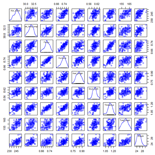
Figure 2. Scatterplot matrix of Bumpus English sparrow traits. Traits were (left-right): Alar extent (mm), length (tip of beak to tip of tail), length of head (mm), length of femur (in.), length of humerus (in.), length of sternum (in.), skull width (in.), length of tibio-taurus (in.), and weight (g)
R code for graph
car::scatterplotMatrix(~Alar_extent+Beak_head_Length+Femur+Humerus+Keel_Length+Skull_width+Tibiotarsus+Total_length+Weight, regLine=FALSE, smooth=FALSE, diagonal=list(method="density"), data=Bumpus)
Note 2: In Chapter 4, we discussed importance of white space and Y-scale for graphs that make comparisons. Figure 2 is a good example of where we trade-off the need for white space and concerns about telling the story — the various traits are positively correlated — against the dictum of an equal Y-scale for true comparisons.
R packages
factoextra
psa package from MorphoFun/psa/
Rcmdr: Statistics > Dimensional analysis > Principal component analysis …
.PC <-
princomp(~Alar_extent+Beak_head_Length+Femur+Humerus+Keel_Length+Skull_width+Tibiotarsus+Total_length+Weight, cor=TRUE, data=Bumpus)
cat("\nComponent loadings:\n")
print(unclass(loadings(.PC)))
cat("\nComponent variances:\n")
print(.PC$sd^2)
cat("\n")
print(summary(.PC))
screeplot(.PC)
Bumpus <<- within(Bumpus, {
PC2 <- .PC$scores[,2]
PC1 <- .PC$scores[,1]
})
})
Importance of components
                              Comp.1     Comp.2
Standard deviation         2.3046882  0.9988978
Proportion of Variance     0.5901764  0.1108663
Cumulative Proportion      0.5901764  0.7010427
Interpretation
Comp.1 has a significantly higher standard deviation — it captures much more data variation than Comp.2.
Comp.1 explains 59% of the total variation, Comp.2 by itself describes an additional 11% of the variation in the data set. Between the two, 70% of the variation in the data set is explained by just these two components — “high data compression.”
Cluster analysis
Cluster analysis or clustering is a multivariate analysis technique that includes a number of different algorithms for grouping objects in such a way that objects in the same group (called a cluster) are more similar to each other than they are to objects in other groups. A number of approaches have been taken, but loosely can be grouped into distance clustering methods (see Chapter 16.6 – Similarity and Distance) and linkage clustering methods: Distance methods involve calculating the distance (or similarity) between two points and whereas linkage methods involve calculating distances among the clusters. Single linkage involves calculating the distance among all pairwise comparisons between two clusters, then
Results from cluster analyses are often displayed as dendrograms. Clustering methods include a number of different algorithms hierarchical clustering: single-linkage clustering; complete linkage clustering; average linkage clustering (UPGMA) centroid based clustering: k-means clustering.
Cluster analysis is common to molecular biology and phylogeny construction and more generally is an approach in use for exploratory data mining. Unsupervised machine learning (see 20.14 – Binary classification) used to classify, for example, methylation status of normal and diseased tissues from arrays (Clifford et al 2011).
K-means clustering
 -means clustering is an unsupervised learning algorithm that automatically partitions data into
 -distinct, nonoverlapping groups (clusters) based on feature similarity. It finds hidden patterns by iteratively assigning data points to the nearest centroid (mean) and updating the centroids until clusters stabilize.
Ahh, the clusters. The -means problem is to find cluster centers that minimize the sum of squared distances from each data point being clustered to its cluster center (the center that is closest to it). Finding the optimal number of clusters is computationally hard,  hard, because it requires finding the absolute best partition of
 points into clusters, which involves searching an exponential number of possible configurations.
Note 3: hard, where  is short for nondeterministc and
 stands for polynomial time. Interested readers can start at Wikipedia.
Number of clusters
Iterations
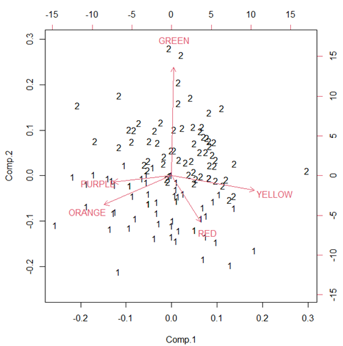
Figure 3. Bi-plot of clusters, Skittles mini bags.
Hierarchical clustering
Ward’s method
Complete linkage
McQuitty’s method
Centroid linkage
A common way to depict the results of a cluster analysis is to construct a dendogram.
Questions
- Write up three learning outcomes for this page. Hint: Point your favorite generative AI to this page and ask for help.
Quiz Chapter 20.6
Dimensional analysis
References and further reading
Bumpus, H. C. (1898). Eleventh lecture. The elimination of the unfit as illustrated by the introduced sparrow, Passer domesticus. (A fourth contribution to the study of variation.). Biology Lectures: Woods Hole Marine Biological Laboratory, 209–255.
Clifford, H., Wessely, F., Pendurthi, S., & Emes, R. D. (2011). Comparison of clustering methods for investigation of genome-wide methylation array data. Frontiers in genetics, 2, 88.
Ferreira, L., & Hitchcock, D. B. (2009). A comparison of hierarchical methods for clustering functional data. Communications in Statistics-Simulation and Computation, 38(9), 1925-1949.
Fraley C, Raftery AE. (2002) Model-based clustering, discriminant analysis, and density estimation. J Am Stat Assoc. 2002; 97(458):611–31.
Ding, C., & He, X. (2004). K-means Clustering via Principal Component Analysis. Proceedings of the 21 St International Conference on Machine Learning.
Vieira, V. M. N. C. S. (2012). Permutation tests to estimate significances on Principal Components Analysis. Computational Ecology and Software, 2.
Chapter 20 contents
- Additional topics
- Area under the curve
- Peak detection
- Baseline correction
- Surveys
- Time series
- Dimensional analysis
- Estimating population size
- Diversity indexes
- Survival analysis
- Growth equations and dose response calculations
- Plot a Newick tree
- Phylogenetically independent contrasts
- How to get the distances from a distance tree
- Binary classification
- Meta-analysis
/MD
2.5 – Scientific method and where statistics fits
- Science isn’t just a recipe.
- Hypothetico-deductive reasoning.
- It’s all about the probability of a particular event.
- A statistical translation of the Scientific Method.
- When we say “experiment,” the hypothesis came first.
- Bottom-up, Top-down.
- How to interpret a test result.
- False discovery rate: claims must be stringently evaluated.
- Projects and the data lifecycle.
- Conclusions.
- Questions.
- Quiz.
- Chapter 2 contents .
Science isn’t just a recipe.
.
The scientific method is what makes science a “powerful way of knowing” (Church and Carpenter 2008), and by now, you should be familiar with the outline: hypothesis, experiment, etc. What distinguishes science from other fields of inquiry is that at its best, science accumulates verifiable evidence about our world. I begin with a disclaimer — our introductory textbooks tend to reify the scientific method (cf. Blachowicz 2009). Outside of the classroom and introductory science text books, I don’t think you’ll find much agreement among practicing scientists precisely what the scientific method entails, or whether strict adherence to a list of steps distinguishes what scientists do compared with other professions. For one difference, typical discussions of the scientific method may emphasize the experiment, which probably brings to mind images of a lab coat and test tubes, but should emphasize the critical thinking “tool kit” (Wivagg and Allchin 2002), eg, model-based inquiry. That said, holding a view that introductory textbooks should present nuances of epistemology seems a big ask.
But we do emphasize experimentation with good reason. In principle it is straightforward to identify what control groups are needed to conduct an experiment in the lab, but what are the control groups for an experiment conducted on the computer? In most cases, one should argue that if an outcome is obtained by random processes, then no additional cause need be addressed. Therefore, the control group for a simulation would be a random process generator.
Disagreements about the scientific method center about how science is really done (eg, from a social perspective), but also because there appear to be differences in approach in sciences that work on historical questions (physical cosmology, evolutionary biology, geology), and those that conform to the classic experimental approach (chemistry, molecular biology, physics). Epistemology is a fascinating area — How do we know what we know, What exactly is science and how is it different from other areas of knowing, etc. But I will leave you only with the tantalizing suggestion to read more and start with you with a list of readings to start (see Readings below). This is the stuff of graduate and professional school; we have work to do.
Despite apparent differences between what scientists say they do and how they actually do sciences, there is broad agreement; science as a way of knowing can be characterized by the following steps (National Academy of Sciences 1999).
- Begin with facts, which are observations confirmed and treated as true
- Formulate a hypothesis, with emphasis on hypotheses that are testable statements about relationships observed about the natural world
- Given the possible outcomes, state predictions derived from the hypothesis.
- Make observations of perform an experiment designed to test the hypothesis.
- Analyze the data from the experiment.
- Evaluate the results of the experiment against the predictions.
- Repeat.
This deceptively simple list hides much work to be done. Hypotheses are not “educated guesses,” where educated guess implies an idea about some phenomenon is likely the correct explanation because of the skill or knowledge of the person making the guess. Good hypotheses make possible experimental tests whose results can be used to rule out alternative explanations, sensu Platt’s “strong-inference”.
Hypothetico-deductive reasoning.
.
I mention this disclaimer about the common (and reassuring) textbook discourse on the scientific method to suggest that, if you have not already reached this point in your career, it is time to move past the cookbook approach to thinking about what it means to do science in practice. Yet another helpful reading is from a paper in Environmental Health by Ozonoff amd Grandjean (2020).
In other words, what makes “good science”?
There is induction and deduction and probabilistic thinking that must be grappled with, all emphasizing efforts by the individual, and yet science, if it is to make any progress must ultimately be a communal activity (Varmus 2009). In particular, to the extent a researcher consistently applies hypothetico-deductive reasoning, or as Platt (1964) called it, “strong-inference,” then good science can happen (see Fudge 2014 for an update). Strong inference according to Platt implies that researchers should follow three steps (after Fudge 2014):
- develop alternative hypotheses
- think of a crucial experiment that can exclude one or more hypotheses
- perform the experiment and obtain a clean result.
Then, beginning with step 1, repeat the procedure to refine the possibilities that remain.
The list of elements of the scientific method neglected to address the crucial role of scientists engaged in an active community of scientists fits in. However, we can can quickly suppose that every step of the scientific method can involve input from others to help shape, improve, and indeed carry out the activities needed to practice science. What scientists share is critical thinking and the tools of statistics provides a common language.
It’s all about the probability of a particular event.
.
Platt (1964) wrote that the observations we make that are puzzling or hard to explain, which implies our understanding is incomplete. We then proceed to ask questions about why the observations are different from our expectations, and we speculate about how the outcome comes about. Thus, we have to consider the probability, or chance, of a particular outcome (event) compare to other possible outcomes. Statistics is about analyzing the probability of outcomes. But there is a twist; there are two distinct, but complementary approaches to statistics. Most of the statistics you have been taught so far comes from the frequentist approach. That is, how often (frequency) will we get the kind of results we observe given the hypothesis? Another approach can be termed Bayesian, where the question is how likely is the hypothesis to be correct given the data? These two approaches view the data obtained from the same experiment differently. A frequentist views the data as random — repeat the experiment and the results will differ — but the hypothesis is fixed (it is either true or it is not). A Bayesian on the other hand views the hypothesis as random with a probability of being true somewhere between zero and 100 percent and the data are fixed.
Which are you, a frequentist, or a Bayesian? Consider the following from xkcd.com no. 1132 (Fig. 1).
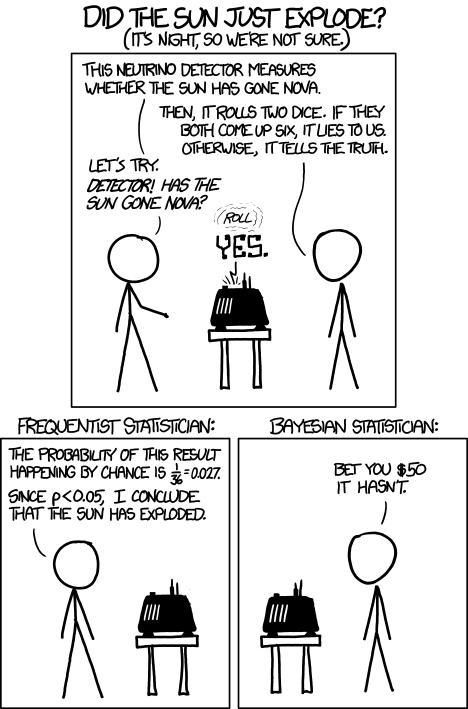
Figure 1. “Frequentists vs Bayesians,” xkcd.com no. 1132
The Bayesian approach makes sense when there exists prior knowledge — the Sun came up this morning, as it did the day before, and the day before that, etc. New data are assessed against what we already know. The Frequentist approach, despite philosophical shortcomings, works for analyzing experiments where prior knowledge is lacking about outcomes. Because much of biomedical research is based on the Frequentist approach, most of our efforts, too, will utilize that approach.
A statistical translation of the Scientific Method.
.
Given our frequentist perspective, we can outline our Scientific Method as follows.
- Formulate a Null and an Alternative hypothesis.
- State predictions from the Null and an Alternative hypotheses.
- Design an experiment or observation.
- Analyze the data from the experiment or observation.
- Interpret the experiment or observation.
- Evaluate the predictions from the Null and an Alternative hypotheses.
- Accept (provisionally) or reject (provisionally) the Null hypothesis.
- Evaluate model fit and robustness
- Repeat.
In practice, there is more to statistics than these 8(9) steps, but this does provide the outline of what statistical analyses are about. There are nuances to how a Frequentist or a Bayesian views statistical analyses as evidence for or against a conclusion (Goodman 1999a, 1999b). We need to distinguish between when data are acquired in the process; data may come before or after the hypotheses are stated. In epistemology, hypotheses are either a priori or a posterori and we need to add these to our discussion of Scientific Method. The terms are Latin, translated apparently as “from the earlier” and “from the later, respectfully.
Note from the lists described as “the” scientific method how hypothesis comes first. Folks who think and write about how and why we know what we know — the discipline is called epistemology — tell us we are generally on more solid footing when we design experiments with specific intent, specific and testable hypotheses. The branch of statistics concerned with experimental design provides rich context for many practical aspects of how to implement experiments — in other words, how to follow the Scientific Method, even if turns out there isn’t just one universal definition of Scientific Methods out there.
When we say “experiment,” the hypothesis came first.
.
More commonly in statistics, the phrases planned, and therefore a priori, and unplanned or a posterori, comparisons are referenced. In practice, biologists design experiments and make observations accordingly to test one or more hypotheses, but they may also address additional hypotheses after the fact. Especially if the experiment generates a lot of data.
You may have also heard of the phrase data mining. Data mining is loosely defined, but mostly refers to sets of protocols and procedures to extract patterns from large data sets stored in databases. Google apparently does lots of data mining as do many other businesses that obtain large amounts of data. Unplanned comparisons includes any data mining protocols, no matter how sophisticated the language sounds (feature selection, classification tree). Data mining is not consistent with classic experiments; it’s different than Step 6 (Step 8 in the second list) listed above because no new data or experiment is carried out.
Can you get away with coming up with and testing new hypotheses from data gathered from an experiment designed to test a different hypothesis? Yes, and of course, the process can be quite profitable for Google. However, you should proceed with caution and restraint. If you are not careful about how you write it up — you will probably be called on it by a reviewer of your work. Is this a posterori approach still science? Of course, yes! I’d even go so far as to say that when one studies real systems, you can’t limit yourself to only planned hypotheses and testing. At least, one designs experiments and carries out those tests but then also uses current data to generate new ideas. Science is also exploratory — you may not design an experiment at all, but through observations, you probably will develop testable hypotheses! We’ll return to these concepts soon. What you must be aware of in any unplanned comparison or data mining sojourn is the possibility of committing a data dredging (aka p-hacking) sin — searching through data to come up with misleading, but statistically “significant” results (Ioannidis 2007; Stefan and Schönbrodt 2023).
Testing of unplanned a posterori hypotheses is a real concern in science. On the one hand, those who think about how we learn about the world and make sense of it have stated emphatically that the best way we know is to follow the scientific method — and that begins with hypotheses followed by designed experiments to test claims derived from those a priori hypotheses. We (teachers, textbook author) continue to teach science as the act of individuals toiling away in the forest or in the lab, pursuing sets of questions that may involve the collection of measurements on dozens to a few hundred subjects. While this type of science is still in practice, there is no doubt that big science involving many people is more common and, perhaps, better at generating new knowledge (Wuchty et al 2007). One result of “big science” is to generate a lot of data, the very essence now of big data, and there must be room for testing of new hypotheses gathered on data sets. This is the essence of the argument for the ENCODE project (ENCODE Project Consortium 2012) — generate lots of genetic data on the human genome using common techniques and make the data publicly available — new research can be conducted on old data.
Bottom-up, top-down.
.
Consider the pronouncements (almost daily it seems!) about the discovery of a new gene for some disease, process, or behavior in humans. Often times, although not always, these “discoveries” are not duplicated by other research groups. Why not? Well, for one, the phrase “gene for” is a dubious shorthand for what is usually a more complex causation. But from our statistical perspective it is problematic because the search for genes is really an a posterori exercise — one begins with phenotypic differences (some have the disease, others do not) and some genetic information (SNPs, DNA sequencing) and then proceeds to see if there are any differences in the genetic material at hand between the two groups. This approach, the Genome Wide Association Study, or GWAS, would be termed “top-down” — begin with the phenotypic differences and search for genetic differences between those that do and those who do not have the condition. Sampling is an issue (are the unaffected subjects a random sample from the entire population?), but the problem also is one of logical design — the hypothesis is made after the fact — a statistical difference between the groups is attributed to a particular genetic difference.
Case-control subjects, where patients with the condition are matched with other individuals who do not have the condition, but match in other ways (eg, age, income, etc.), are enrolled in such studies because there can be no random assignment of subjects to treatment. Case-control subjects are selected such that affected and unaffected individuals are matched by characteristics in as many meaningful ways as possible (eg, age, gender, income, etc.). Because many tests are conducted in GWAS studies, ie, is there a difference between the control and affected group for the first gene, the second gene, and so on up to the number of genes on the microarray chip (10,000 or more genes), the chance that any particular association is a false positive is high, discussed further when we cover Risk Analysis in Chapter 7.
How to interpret a test result.
You are a medical doctor reading the results of a test for three-month average glycated hemoglobin, A1C, levels for your patient. For example, A1C above 6% is considered strong marker of diabetes. A marker, yes, but not the same as a guarantee that a person has diabetes. A false positive (FP) is the case where a test result is positive, but the subject in fact does not have the condition. False positive is equal to the ratio of

where FP is number of false positive readings and TN refers to the true negative, those who in fact do not have the condition.
In Chapter 7 we will spend some time on risk analysis. To introduce this important subject in biostatistics, we’ll begin with an example. A study of 15,934 subjects without diagnosed diabetes found 3.8% or 605 individuals had elevated A1C levels, or about 7.1 million adults not yet diagnosed with diabetes (Selvin et al 2011). About 90% of these individuals also had fasting glucose levels greater than 100 mg/dL, i., diabetic. This is clearly a good test. However, note that 10% of the 605 individuals had elevated A1C, but fasting glucose levels less than 100 mg/dl, ie, did not meet the diagnostic of type 2 diabetes. Thus, the false positive rate is about 0.4%, or nearly 30,000 adults with elevated A1C without diabetes.
Working through frequencies can be challenging, so applying a natural number approach helps. Having just read through the frequencies and percentages, now look at how they translate to probability tree (Fig. 2). Start by utilizing a per capita rate standard: for proportions in the 10 – 20% range, a standard 1000 persons works well (Fig. 2).
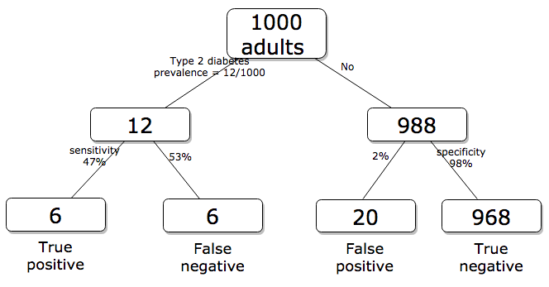
Figure 2. Probability tree diagram with prevalence of type 2 diabetes and sensitivity, specificity of A1C test, data from CDC and Selvin et al 2011. Tree drawn with free diagrams.net app.
How many expected to have A1C above 6%? Twenty-six total positives, only 23% are true positives. An important lesson is that if the prevalence of a condition is low, then any diagnostic test with high sensitivity necessarily will identify many false positives.
False discovery rate: claims must be stringently evaluated.
.
The genome scientists involved in GWAS studies generally are aware of false positives, also termed false discovery rate (FDR), conduct statistical corrections to account for false positives (eg, Brzyski et al 2016), and generally are cautious in their interpretation. But not always. Studies of associations between autism and environment come to mind (eg, Waldman et al 2008), and recent developments in the direct-to-consumer genetic testing market also suggest that the limitations of these kinds of studies are not always represented.
There is a broader concern about the reliability of research, and the debate about how to improve reliability comes from a call to understand how to do statistics better and, more importantly to understand how statistics are to be used in making claims from statistical results (Ioannidis 2007; but see Goodman and Greenland 2007). A key element of scientific work is that findings are repeatable: results from one group should apply to other groups. One dictate to improve reproducibility — increase number of subjects in studies — is obvious, but given the cost of GWAS, currently an unreasonable demand.
In some cases, biologists already have a particular gene in mind, whose function is more or less known, and then the exercise follows the Scientific Method listing much more directly. This bottom-up approach leads to a straightforward, testable genetic hypotheses: a specific difference in genomic sequence predicts a difference in phenotype outcome. A good example is the identification of more than 100 different single nucleotide mutations, called single nucleotide polymorphisms or SNPs, in the CFTR gene of patients known to have cystic fibrosis disease (Castellani 2013). As of August 2018, the number of known pathogenic or likely pathogenic SNPs is now listed at 440 in the SNP database; to put this in some context, there are more than 40,000 reported single nucleotide polymorphisms for the CFTR gene (this number includes SNP duplicates).
Projects and the data lifecycle.
A requirement for our biostatistics course, students are asked to design and implement a research project during the semester (Hydorn 2019). The project can either be part of an ongoing student research project or solely confined to the biostatistics course. The topics are diverse, ranging from observational to experimental to systematic reviews from the disciplines of biology, environmental science, and public health. Examples of project ideas implemented in the biostatistics and related courses at Chaminade University include:
- effects of environmental stress on growth rates.
- 2D and 3D shape analysis of mollusk shells.
- Individual variation and fluctuating asymmetry of plant leaves and flowers along an altitudinal gradient
- several systematic reviews (meta analysis) of published works of interest to public health
- vaccination benefits and risks.
- pain management of over the counter vs prescription medication.
- efficacy of “alternative medicine” approaches to health.
- comparisons of types of medical insurance on patient outcomes of knee replacement therapy.
The justification for the project learning activity is that it provides hands-on opportunity to apply statistical and data sciences concepts to real-world problems. Students work through the challenges of developing a research question, identifying testable hypotheses, designing a study, collecting data, performing analysis, and interpreting results. Importantly, students must decide for themselves which statistical tests and methods are most appropriate for their unique data, rather than simply following a formula presented in a lecture. This connects abstract statistical ideas to practical application, promoting a deeper, more lasting understanding. We manage the projects by encouraging a research lab community: students discuss with their peers their ideas, their data collection and experimental design challenges, with the instructor serving to guide and mentor the multiple projects and intervene as needed to steer student projects towards completion.
Throughout the semester we model the project approach. Students are encouraged to create a working folder on their computer, while dividing homework and other assignments into named projects. Students are also asked to address aspects of their project’s data life cycle (Borgman 2019, Ezer and Whitacker 2019, Griffin et al 2018). A quick Google search on the phrase returns millions of hits (see Note 1), but key elements of the concept are that projects have a beginning and an end, and it is helpful — and in the case of our statistics course, required — to address project management.
Note 1: For example, “8 Steps in the Data Life Cycle,” by Tim Tobierski of Harvard Business School.
BI-311 students, see Homework 1: Project data life cycle in Mike’s Workbook for Biostatistics.
Projects include data generation and collection, data processing, storage and data management, data exploration and visualization, interpretation and reporting. Thus, students need to develop a data management plan, which includes how data are collected, application of best practices to insure data file and storage of images, and how to share the project results. We ask students to develop 10-min research talks, which are presented and recorded, suitable for ePortfolio inclusion.
Conclusions.
.
Epistemology, the theory of how knowledge is acquired, is a complicated business – what I want you to appreciate now is that planned and unplanned comparisons affect interpretation of your statistical results, how the difference is likely also to affect the reproducibility of your work. In the language or clinical trials and experimental design, planned and unplanned accompany prospective and retrospective studies (Chapter 5). A prospective study in the case of GWAS means genetic differences among individuals are known at the start of the study, and phenotypic differences arise naturally during the course of the study. Knowing the strengths and limitations of, for example, a planned retrospective study is at the heart of experimental design (Chapter 5).
In the biostatistics course, students are required to design and carry out an independent research project that integrates statistical methods with real-world problems in biology, environmental science, or public health. The course emphasizes hands-on learning through the full research process—from formulating questions to data collection, analysis, and interpretation—while fostering a collaborative research lab environment. Students also learn project and data management skills and conclude by presenting their findings in recorded research talks suitable for inclusion in an ePortfolio.
Questions.
- Write up three learning outcomes for this page. Hint: Point your favorite generative AI to this page and ask for help.
- Above we described how GWAS studies are generally top-down; What would constitute a bottom-up approach to GWAS?
- In your own words provide pro and con points of view on data mining of large data sets.
- Create a stylized infographic, like a mind map, to illustrate the data life cycle for a one semester research project.
Quiz Chapter 2.5
Scientific method and where statistics fits
Chapter 2 contents
.
2.3 – A brief history of (bio)statistics
Foundations of biostatistics: key definitions.
.
Before discussing history and landmark moments in biostatistics, let’s start with basic definitions.
Bioinformatics is loosely defined as a discipline of biology primarily concerned with work involving large data sets (eg, databases), but a bioinformatician would not primarily be a statistician necessarily. Rather, a bioinformatician in addition to foundation in statistical and mathematical training would likely be fluent in at least one programming language and confident in use and design of databases.
Biostatistics, or biometry, then, refers to use of statistics in biology. Biostatistics encompasses application of statistical approaches to design, analyze, and interpret biological data collected through observation of use of experimentation. In turn, there are many broad disciplines or fields of specialty that trained biostatisticians may work.
Chance, the likelihood that a particular event will occur.
Data scientist, a very general label, is a person likely to work on “big data.” Big data may be loosely and inconsistently identified as access to large detailed and unstructured data sets such as visits and behavior within websites of tens of millions of Internet “hits” to a website like Amazon® or Google®. The data scientist would then be involved in extracting meaning from volumes of this data in a process called data mining. In the context of biology web sites like allele frequency aggregator at NCBI, which houses allele frequency information collected on human populations, the 1000 genome project, or any of the databases accessible at National Center for Biotechnology Information would constitute sources of big data for biological researchers.
Epidemiology refers to the statistics of patterns of and risk of disease in populations, particularly of humans and thus, an epidemiologist would also be considered to be a biostatistician. The statistics of epidemiology include all of the materials we will cover in this course, but perhaps if any particular analytical approach characterizes epidemiology, it would be survival analysis (review in Clark et al 2003) — in competition with compartment models to predict spread of communicable disease in populations (Brauer 2017).
Event, an outcome to which a probability is assigned.
Likelihood, the probable chance of occurrence of an event that has already occurred. Likelihood assesses how well a particular model or set of parameters explains observed data.
Probability, the chance that an event will occur in the future, given a known model or set of parameters.
Random or random chance. This is a good place to share a warning about vocabulary; statistics, like most of science, uses familiar words, but with refined and sometimes different meanings than our everyday usage. Consider our everyday use of random: “without definite aim, direction, rule, or method – subjects chosen at random” (Merriam-Webster online dictionary). In statistics, however, random refers to “an assignment of a numerical value to each possible outcome of an event” (Wikipedia, Eagle 2021). Thus, in statistics, random dictates a method of determining how likely a subject is to be included: If represents the size of the population, then random sampling implies that each individual had  chance of being selected. Thus, if
 , then each individual has a 1% (
 ) chance of selection. This is quite different from Merriam-Webster’s definition, in which no method is assumed. To a statistician, then, random as used in everyday conversation would imply haphazard sampling or convenience sampling from a population.
Statistics may be defined as the science of collecting, organizing, and interpreting data. Statistics is a branch of applied mathematics. Note that the word statistic is also used, but refers to a calculated quantity like the mean or standard deviation. A little confusing, but the context in which statistics or statistic is appropriate is usually not a major issue.
Note 1. Did you notice how the definitions for chance, likelihood, and probability were rather circular? Of the three, chance is more informal while both likelihood and probability are distinct concepts in statistics.
From dice games to data science: A brief history of statistics.
.
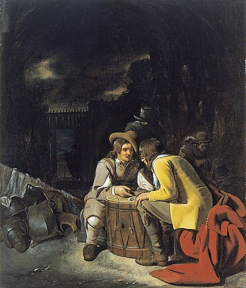
Figure 1. Soldiers playing dice, painting by Michiel Sweerts (1618–1664). Public domain image, https://commons.wikimedia.org/
The concepts of chance and probability, so crucial to statistical reasoning — because it allows us to interpret data when outcomes are inconsistent — were realized rather late in the history of mathematics. While people have been writing about applied and theoretical math for thousands of years, probability as a topic of interest by (Western) scholars seems to date only back to the late 17th century, beginning with letters written between Pierre de Fermat (1601-1665) and Blaise Pascal (1623 – 1662) and the substantial work on probability by Pierre-Simon Laplace (1749-1827). Often, research on probability developed under the watchful eyes of rich patrons more interested in gaming (sensu Fig 1), than to scientific applications. Work on permutations and combinations, essential for an understanding of probability, trace to India prior to Pascal’s work (Raju 2011).
The history of statistics goes back further if you allow for the dual use of the term statistics, both as a descriptor of the act of collecting data and as a systematic approach to the analysis of data. Prior to the 1700s, statistics was used in the sense of collection of data for use by the governments. It is not until the latter part of the 19th century that we see scholarship on statistical analytical techniques. Many of the statistical approaches we teach and use today were developed in the decades between 1880s and the 1930s. Work by Francis Galton (1822-1911), Karl Pearson (1857-1936), RA Fisher (1890-1962), Sewall Wright (1889-1988), Jerzy Neyman (1894-1981), Egon Pearson (1895-1980, Karl Pearson’s son), George EP Box (1919-2013) remains highly influential today.
Development of randomized controlled (clinical) trials, RCT, the “gold standard,” by the 1950s provides the strongest study design to evaluate the effectiveness of clinical or other kinds of interventions. The general features of RCT are (1) comparison among groups, with at least one control group, (2) randomization, and (3) blinding, where treatment options are concealed from the subjects (single-blind) and from those charged to assess the outcomes (double-blind). Sir Austin Bradford Hill (1887-1991) is generally credited with developing the RCT (Collier 2009, Matthews 2016), but we owe RA Fisher for randomization in experimental design. Hill (1965) is also known for Hill’s criteria of causality — nine principles that can be used to establish causal relationship between epidemiological (observational) evidence and disease. Chief among these nine principles are strength of the association (effect size) and consistent association (reproducibility), elements we return to often in our introduction to biostatistics.
Since the 1950s, there has been an explosion of developments in statistics, particularly as related to power of computer. These include use of resampling, simulation, and Monte Carlo methods (Harris 2010). Resampling — the creation of new samples based on a set of observed data — is a key innovation in statistics. Its use led to a number of innovative ways to estimate the precision of an estimate (see Chapter 3.4 and Chapter 19). Monte Carlo methods, or MCM, which involves resampling from a probability distribution, is used to repeat (simulate) an experiment over and over again (Kroese et al 2014). Computers have so influenced statistics that some now define statistics as “…the study of algorithms for data analysis” (p 175, Beran 2003). So much so, the role of computers and coding to process and model data, we now have the discipline of Data Science. For more on the history of statistics, see Anderson (1992), Fienberg (1992), and Freedman 1999; for excellent, conversational books read Salsburg (2002) and McGrayne (2011). For influential women in early development of statisticians, see Anderson (1992).
Numbers and prejudice: A hidden history of statistics.
.
Many statistical methods in use today, including regression and analysis of variance methods, can trace their origins to the late 1800’s and early 1900’s (Kevles 1998). Many of these early statisticians developed statistical methods to, at least in part, further their interests in understanding differences between racial groups of humans. Sir Francis Galton, who developed regression and correlation concepts (the details and extensions of which were the works of Karl Pearson), coined the term Eugenics, the “science” of improving humans through selective breeding. In an editorial, the journal Nature recently published an apology for it’s complicity providing “a platform to [eugenicists] views” (p 875, Nature 2022). Sir RA Fisher is rightfully remembered as the inventor of analysis of variance and maximum likelihood techniques (Rao 1992; Bodmer et al 2021), and perhaps more important, developed the concepts of sampling from populations, degrees of freedom, among other contributions. Moreover, work of Fisher, Wright, and others led to the realization that populations of the same species differed at many locations in the genome, thus completely refuting any notion of “racial purity” (Bodmer et al 2021). However, Fisher was an active promoter of eugenics (Bodmer et al 2021), and an award given by The Society for the Study of Evolution in his honor, the RA Fisher Prize, was renamed in 2020.
Eugenics is still with us (Liscum and Garcia 2022; see also Legacies of Eugenics: An Introduction Los Angeles Review of Books; Veit et al 2021), but the era of “Three generations of imbeciles are enough” (Buck v. Bell), and the forced sterilization eugenic programs of the Nazi (Kelves 1999), were thoroughly discredited on scientific grounds many times (click here for Eugenics Archive website). Do keep in mind that the times were different, and elements of eugenics thinking remains with us (cf discussion in Veil et al 2021 and references therein), it is interesting nevertheless to learn about the murky history of statistics and the objectives of some of the very bright people responsible for many of the statistical analyses we use today (see Stephen J. Gould’s “The Mismeasure of Man“). Several books tackle aspects of scientific racism, including 2017 Is science racist? by Jonathan Marks and 2019 Superior: The return of of race science, by Angela Saini, Cathy O’Neil’s 2017 accessible book Weapons of math destruction: How big data increases inequality and threatens democracy, and a host of articles and books listed at Wikipedia.
Keep in mind also that geneticists and statisticians were instrumental in showing why Eugenics was unscientific, at best. See partial listing in Bodmer et al (2021). Also, see 2021 review by Rebecca Sear, Demography and the rise, apparent fall, and resurgence of eugenics, in Population studies: A journal of demography. While the algorithms of statistics should be unbiased — and we often believe that they are — clearly, humans, and the interpretations of data may be biased (Celiktutan et al 2024). Statistical reasoning absolutely requires considering sources of bias and their impacts on our conclusions.
Landmark epidemiology studies.
.
John Snow (1813-1858) is credited by some as the “Father of Epidemiology”(Ramsay 2006). During a London outbreak — the sudden increase of disease events — of cholera in 1854, Snow conducted work to establish cholera mortality with source and quality of drinking water. At the time, the prevailing explanation for cholera was that it was an airborne infection. Snow’s map of cholera mortality in the Golden Square district of London in relation to a water pump on Broad Street is shown in Fig 2, Snow’s theory of contaminated water was not accepted as an explanation for cholera until after his death.
Original map by John Snow showing the clusters of cholera cases in the London epidemic of 1854, drawn and lithographed by Charles Cheffins.
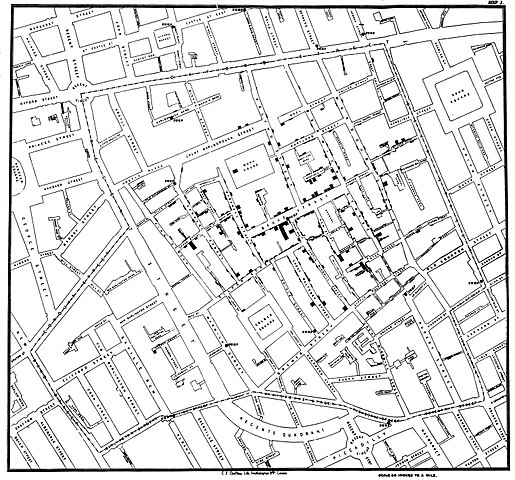
Figure 2. Original map by John Snow showing the clusters of cholera cases in the London epidemic of 1854, drawn and lithographed by Charles Cheffins. Image Public Domain, from Wikipedia.

Snow’s work and dataset can be viewed and thanks to Paul Lindman and others, the work can be expanded: for example, define areas around pumps by walking distance (Fig 3). The R package is cholera. Figure 2 shows a plot like Snow’s annotated map.cholera.
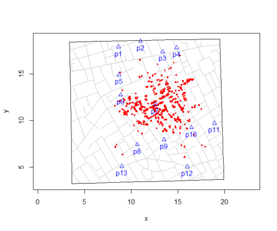
Figure 3. Plot of Snow’s London using R cholera package. Triangles marked with p1-p13 represent public water pumps. Red dots represent cholera cases.
R code to make the plot was
snowMap()Snow’s ideas about cholera were not accepted in his time and you should recognize that by itself, a cluster map supports both the airborne and waterborne theories. The cholera package contains additional data to help visualize the area, including setting regions by walking distance (Fig 4).
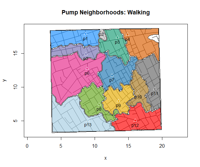
Figure 4. Plot of Snow’s London with walking areas drawn about the 13 water pumps. R cholera package.
R code to make the plot was
plot(neighborhoodWalking(case.set = "expected"), "area.polygons")Epidemiology of cancer.
.
This is an undeveloped section in my book. For now, I’ve listed a number of key landmark studies — a selective and incomplete list — in the history of epidemiology and cancer risk — these would serve well as case studies:
- Tobacco as a carcinogen
- Doll R, Hill AB. Smoking and carcinoma of the lung; preliminary report. Br Med J 1950; 2: 739–748
- Fontham ET, Correa P, Wu-Williams A, Reynolds P, Greenberg RS, Buffler PA, Chen VW, Boyd P, Alterman T, Austin DF, Liff J, Greenberg SD. Lung cancer in non-smoking women: a multicenter case-control study. Cancer Epidemiol Biomarkers Prev 1991;1:35-43
- Diet and cancer risk
- Kolonel LN, Hankin JH, Lee J, Chu SY, Nomura AM, Hinds MW. Nutrient intakes in relation to cancer incidence in Hawaii. Br J Cancer 1981;44:332-339.
- Obesity, exercise, and cancer risk
- Calle EE, Rodriguez C, Walker-Thurmond K, Thun MJ. Overweight, Obesity, and Mortality from Cancer in a Prospectively Studied Cohort of U.S. Adults. N Engl J Med 2003;348:1625-1638.
- Hormones and cancer risk
- Marchbanks PA, McDonald JA, Wilson HG, Folger SG, Mandel MG, Daling JR, Bernstein L, Malone KE, Ursin G, Strom BL, Norman SA, Wingo PA, Burkman RT, Berlin JA, Simon MS, Spirtas R, Weiss LK. Oral contraceptives and the risk of breast cancer. New Engl J Med 2002;346(26):2025-2032.
- Cancer risk and occupations
- absence of cervical cancer but high incidence of breast cancer in nuns (Ramazzini, 1713)
- cancer of the scrotums among chimney sweeps of London (Pott, 1775)
- Silverman DT, Hoover RN, Mason TJ, Swanson GM. Motor exhaust-related occupations and bladder cancer. Cancer Res 1986;46:2113-2116.
Please see review by Greenwald and Dunn (2009).
Questions
- Write up three learning outcomes for this page. Hint: Point your favorite generative AI to this page and ask for help.
- Expand my example of landmark studies (also called pivotal or seminal studies) in epidemiology of cancer to a subject of your own interest. For example, vaccination and communicable diseases like polio.
.
Quiz Chapter 2.3
A history of (bio)statistics
Chapter 2 contents
.
- Introduction
- Why biostatistics?
- Why do we use R Software?
- A brief history of (bio)statistics
- Experimental Design and rise of statistics in medical research
- Scientific method and where statistics fits
- Statistical reasoning
- Chapter 2 – References and suggested reading
4 – How to report statistics
Introduction: Reporting your results.
While you are thinking about exploring data sets and descriptive statistics, please review our overview of data analysis (Chapter 2.4 and 2.5). While the scientific hypotheses come first, how experiments are designed should allow for straight-forward analysis: in other words, statistics can’t rescue poorly designed experiments, nor can it reveal new insight after the fact.
Once the experiments are completed, all projects will go through a similar process:
- Description: Describe and summarize the results.
- Check assumptions.
- Inference: conduct tests of hypotheses.
- Develop and evaluate statistical models.
Clearly this is a simplification, but there’s an expectation your readers will have about a project. Basic questions like how many subjects got better on the treatment? Is there an association between Body Mass Index (BMI) and the primary outcome? Did male and female subjects differ for response to the treatment? Undoubtedly these and related questions form the essence of the inferences, but providing graphs to show patterns may be as important to a reader as any p-value — a number which describes how likely it is that your data would have occurred by chance — eg, from an Analysis of variance.
Each project is unique — sorry, what a breathtakingly obvious statement — but what elements must be included in a results section?
Data visualization.
We describe data in three ways: graphs, tables, and in sentences. In this page we present the basics of when to choose a graph over presenting data in a table or as a series of sentences (ie, text). In the rest of this chapter we introduce the various graphics we will encounter in the course. Chapter 4 covers eight different graphics, but is by no means an exhaustive list of kinds of graphs. Phylogenetic network graphs are presented in Chapter 20.11. Although an important element of presentation in journal articles, we don’t discuss figure legends or table titles; guidelines are typically available by the journal of choice (eg, PLOS ONE journals guidelines).
A quick note about terminology. Data visualization encompasses charts, graphs and plots. Of the three terms, chart is the more generic. Graphs are used to display a function or mapping between two variables; plots are kinds of graphs for a finite set of points. There is a difference among the terms, but I confess, I won’t be consistent. Instead, I will refer to each type of data visualization by its descriptive name: bar chart, box plots, histograms, scatter plot, etc. Note that technically, a scatter plot can refer to a graph, eg, a line drawn to reflect a linear association between the two variables, whereas bar charts and box plots would not be a graph because no function is implied.
Why display data?
Do we just to show a graph to break the monotony of page after page of text or do we attempt to do more with graphs? After all, isn’t “a picture’s worth a thousand words?” In many cases, yes! Graphics allow us to see patterns. Data visualization is a key part of exploratory data analysis (Tukey 1977), or data mining in the parlance of big data (Keim 2001). Data visualization is also a crucial tool in the public health arena, and finding effective graphics to communicate, at times, complex data and information to both public and professional audiences can be challenging (see discussion in Meloncon and Warner 2017).
Graphics are complicated — all the interplay among pixels etc and rendering process — and expensive to do well. Text is much cheaper to publish, even in digital form. But the ability to visualize concepts, that is, to connect ideas to data through our eyes (see Wikipedia), seems to be more the cognitive goal of graphics. Lofty purpose, desirable goal. Yes, it is true that graphics can communicate concepts to the reader, but with some caution. Images distort, and default options in graphics programs are seldom acceptable for conveying messages without bias (Glazer 2011).
Here’s some tips from a book on graphical display (Tufte 1983; see also Camões 2016).
Your goal is to communicate complex ideas with clarity, precision, and efficiency. Graphical displays should:
- show the data
- avoid distorting the data
- present numbers in a small space
- help the viewer’s eye to compare different pieces of data
- serve a clear purpose (description, exploration, tabulation, decoration)
- be closely integrated with statistical and verbal descriptions of a data set.
We accomplish these tasks by following general principles involving scale and a commitment to avoiding bias in our presentation.
Importantly, graphs can show patterns not immediately evident in tables of numbers. See Table 1 for an example of a dataset, “Anscombe’s quartet,” (Anscombe 1973), where a picture is clearly helpful.
Anscombe’s quartet
| X | Y1 | Y2 | Y3 | Y4 |
|---|---|---|---|---|
| 10 | 8.04 | 9.14 | 7.46 | 6.58 |
| 8 | 6.95 | 8.14 | 6.77 | 5.76 |
| 13 | 7.58 | 8.74 | 12.74 | 7.71 |
| 9 | 8.81 | 8.77 | 7.11 | 8.84 |
| 11 | 8.33 | 9.26 | 7.81 | 8.47 |
| 14 | 9.96 | 8.10 | 8.84 | 7.04 |
| 6 | 7.24 | 6.13 | 6.08 | 5.25 |
| 4 | 4.26 | 3.10 | 5.39 | 12.50 |
| 12 | 10.84 | 9.13 | 8.15 | 5.56 |
| 7 | 4.82 | 7.26 | 6.42 | 7.91 |
| 5 | 5.68 | 4.74 | 5.73 | 6.89 |
| Mean (±SD) | 7.50 (2.032) | 7.50 (2.032) | 7.50 (2.032) | 7.50 (2.032) |
The Anscombe dataset is also available in R packages data(Anscombe, package="carData"), or you can copy/paste from Table 1 into a spreadsheet or text file, then load the data file into R (eg, Rcmdr → Load data set). Note that the data set does not include the column summary statistics shown in the last row of the table.
Before proceeding, look again at the table — See any patterns in the table?
Maybe.… Need to be careful as we humans are really good at perceiving patterns, even when no pattern exists.
Now, look just at the last row in the table, the row containing the descriptive statistics (the means and standard deviations). Any patterns?
The means and standard deviations are the same, so nothing really jumps out at you — does that mean that there are no differences among the columns then?
But let’s see what the scatter plots look like before we conclude that the columns of Y ’s are the same (Fig. 1). I’ll also introduce the R package clipr, which is useful for working with your computer’s clipboard.
Note 1: To show clipboard history, on Windows press + V; on macOS, open Finder and select Edit → Show Clipboard.
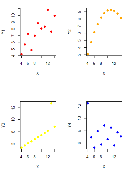
Figure 1. Scatter plot graphs of Anscombe’s quartet (Table 1)
#R code for Figure 1.

require(clipr)
#Copy from the Table and paste into spreadsheet (exclude last row). Highlight and copy data in spreadsheet
myTemp <- read_clip_tbl(read_clip(), header=TRUE, sep = "\t")
#Check that the data have been loaded correctly
head(myTemp)
#attach the data frame, so don't have to refer to variables as myTemp\$variable name
attach(myTemp)
#set the plot area for 4 graphs in 2X2 frame
par(mfrow=c(2,2))
plot(X, Y1, pch=19, col="red", cex=1.2)
plot(X, Y2, pch=19, col="orange",cex=1.2)
plot(X, Y3, pch=19, col="yellow",cex=1.2)
plot(X, Y4, pch=19, col="blue",cex=1.2)
And now we can see that the Y ‘s have different stories to tell. While the summary (descriptive) statistics are the same, the patterns of the association between Y values and the X variable are qualitatively different: Y1 is linear, but diffuse; Y2 is nonlinearly associated with X; Y3, like Y1, is linearly related to X, but one data point seems to be an outlier; and for Y4 we see a diffuse nonlinear trend and an outlier.
So, that’s the big picture here. In working with data, you must look at both ways to “see” data — you need to make graphs and you also need to calculate basic descriptive statistics.
And as to the reporting of these results, sometimes Tables are best (i.e., so others can try different statistical tests), but patterns can be quickly displayed with carefully designed graphs. Clearly, in this case, the graphs were very helpful to reveal trends in the data.
When to report numbers in a sentence? In a table? In a graph?
The choice depends on the message. Usually you want to make a comparison (or series of comparisons). If you are reporting one or two numbers in a comparison, a sentence is fine. “The two feral goat populations had similar mean numbers (120 vs. 125) of kids each breeding period.” If you have only a few comparisons to make, the text table is useful:
Table 2. Data from Kipahoehoe Natural Area Reserve, SW slope of Mauna Loa.
| Location | Number of kids |
|---|---|
| Outside fence | |
| kīpuka | 51 |
| other | 120 |
| Inside fence | |
| kīpuka | 3 |
To conclude, tables are the best way to show exact numbers and tables are preferred over graphs when many comparisons need to be made.
Note 2: A kīpuka is a land area surrounded by recent lava flows. This was a real data set, but I’ve misplaced the citation!
Couldn’t I use a pie chart for this?
Yes, but I will try and persuade you to not. Pie charts are used to show part-whole relationships. If there are just a few groups, and if we don’t care about precise comparisons, pie charts may be effective. Some good examples are Figure 1 O’Neill et al 2020,
Sometimes, people use pie charts for very small data sets (comparing two populations, or three categories, for example). These work well, but as we increase the number of categories, the graphic likely requires additional labels and remarks to clarify the message. The problem with pie charts is that they require interpretation of the angles that define the wedges, so we can’t be very precise about that. Bar charts are much better than pie charts — but can also suffer when many categories are used (Chapter 4.1).
To illustrate the problem, here’s a couple of pie charts from Microsoft Excel (a similar chart can be made with LibreOffice Calc) for our goat data set; compare this graph to the table and to the bar chart below (Fig 2).
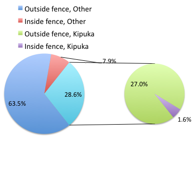
Figure 2. Excel pie chart of Table 2 data set.
A bar chart of the same data (Fig 3).
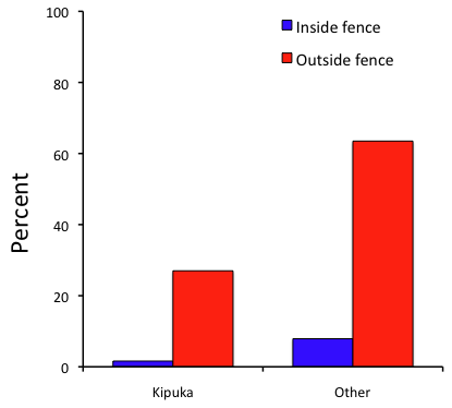
Figure 3. Bar chart of Table 2 data set
The bar chart (Fig 3) is easier to get the message across; more goat kids were found outside the fenced area then inside the fenced in areas. We can also see that more goat kids were found in the “other” areas compared to the kipuka. The pie chart (Fig 2) in my opinion fails to communicate these simple comparisons, conclusions about patterns in the data that clearly would be the take-home message from this project. Aesthetically the bar chart could be improved — a mosaic plot would work well to show the associations in the project results (See Ch 4.4 Mosaic plots). Furthermore, a strong case can be made that the bar chart is over kill — after all, there’s only the four points to show.
Note 3: A much better graph would include the actual counts, eg, a box plot as discussed in Chapter 4.3.
But we are not done with this argument, to use graphics or text to report results. Neither the bar chart (mosaic plot) or the pie chart really work. The reader has to interpret the graphics by extrapolating to the axes to get the numbers. While it may be boring — 1.5 million hits Google search “data tables” boring — tables can be used for comparisons and make the patterns more clear and informative to the reader. Here’s a different version of the table to emphasize the influence of fencing on the goat population.
Table 3. Revised Table 2 to emphasize comparisons between inside and outside the fence line on feral goat population on Mauna Loa.
| Location | Kīpuka | Other |
|---|---|---|
| Outside fence | 51 | 120 |
| Inside fence | 3 | 15 |
Table 3 would be my choice — over a sentence and over a graph. At a glance I can see that more goat kids were found outside of the fenced area, regardless of whether it was in a kipuka or some other area on the mountain side. Table 3 is an improvement over Table 2 because it presents the comparisons in a 2 X 2 format — especially useful when we have a conditional set.
For example, it’s useful to show the breakdown of voting results in tables (numbers of votes for different candidates by voters party affiliation, home district, sex, economic status, etc.). Interested readers can then scan through the table to identify the comparison they are most interested in. But often, a graph is the best choice to display information. One final point, by judiciously combining words, numbers, and images, you should be able to convey even the most complex information in a clear manner! We will not spend a lot of time on these issues, but you will want to pay some attention to these points as you work on your own projects.
Some final comments about how to present data.
What your graph looks like is up to you, lots of people have advice (eg, Klass 2012). But we all know poor graphs when we see them in talks or in papers; we know them when we struggle to make sense of the take-home message. We know them when we feel like we’re missing the take-home message.
Here’s my basic, very subjective take on communicating information with graphics — aka a grammar of graphics, sensu Tufte 2001, and Wilkinson 2005.
- Always include proper labeling: axes, units, legends, and captions.
- Minimize white space (for example, the scatter plots above could be improved simply by increasing the point size of the data points)
- Yes, minimize white space, but always respect the scale, particularly when comparisons are intended.
- Avoid bar charts for comparisons if you are trying to compare more than about three or four things.
- Use color sparingly and with intention: a consistent palette distinguishes groups.
- Avoid overly simple graphs with just a handful of points or bars. Just write it up!
- A graphic in a science report that is worth “a thousand words” probably is too complicated, too much information, and, very likely, whatever message you are trying to convey is better off in the text.
Clever graphics may be visually stunning and, perhaps, serve well to advertise the take home message, but likely they need to be accompanied by a sophisticated text as guide to those take home messages.
Homework to go with this topic.
Homework 2B: Graphs in Mike’s Workbook for biostatistics.
Quiz
In addition to ten general questions in quiz-form about this page contents, a total of 94 questions among the several subchapters, a mix of true or false and multiple choice question format.
Quiz Chapter 4
How to report statistics
Chapter 4 contents