17.5 – Testing regression coefficients
Introduction
Whether the goal is to create a predictive model or an explanatory model, then there are two related questions the analyst asks about the linear regression model fitted to the data:
- Does a line actually fit the data
- Is the linear regression statistically significant?
We will turn to the first question pertaining to fit in time, but for now, focus on the second question.
Like the one-way ANOVA, we have the null and alternative hypothesis for the regression model itself. We write our hypotheses for the regression
H0 : linear regression fits the data vs. HA : linear regression does not fit
We see from the output in R and Rcmdr that an ANOVA table has been provided. Thus, the test of the regression is analogous to an ANOVA — we partition the overall variability in the response variable into two parts: the first part is the part of the variation that can be explained by there being a linear regression (the linear regression sum of squares) plus a second part that accounts for the rest of the variation in the data that is not explained by the regression (the residual or error sum of squares). Thus, we have

As we did in ANOVA, we calculate Mean Squares  , where x refers to either “regression” or “residual” sums of squares and degrees of freedom. We then calculate F-values, the test statistics for the regression, to test the null hypothesis.
The degrees of freedom (DF) in simple linear regression are always

where
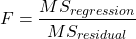
and FDFregression, DFresidual are compared to the critical value at Type I error rate α, with DFregression, DFresidual.
Linear regression inference
Estimation of the slope and intercept is a first step and should be accompanied by the calculation of confidence intervals.
What we need to know if we are to conclude that there’s a functional relationship between the X and Y variable is whether the same relationship exists in the population. We’ve sampled from the population, calculated an equation to describe the relationship between them. However, just as in all cases of inferential statistics, we need to consider the possibility that, through chance alone, we may have committed a Type I error.
The graph below (Fig 1) shows a possible outcome under a scenario in which the statistical analyst would likely conclude that there is a statistically significant linear model fit to the data, but the true relationship in the population was a slope of zero. How can this happen? Under this scenario, by chance alone the researchers sampled points (circled in red) from the population that fall along a line. We will conclude that there is linear relationship — that’s what are inferential statistics work would indicate — but there was none in the population from which the sampling was done; there would be no way for us to recognize the error except to repeat the experiment — the principal of research reproducibility — with a different sample.
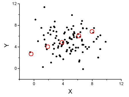
Figure 1. Scatterplot of hypothetical x,y data for which the researcher may obtain a statistically significant linear fit to sample of data from population in which null hypothesis is true relationship between x and y.
So in conclusion, you must keep in mind the meaning of statistical significance in the context of statistical inference: it is inference done on a background of random chance, the chance that sampling from the population leads to a biased sample of subjects.
Note 1. If you think about what I did with this data for Figure 1 graph, purposely selecting data that showed a linear relationship between Y and X (red circles), then you should recognize this as an example of data dredging or p-hacking, cf. discussion in Head et al (2015); Stefan and Schönbrodt (2023). However, the graph is supposed to be read as if we could do a census and therefore have full knowledge of the true relationship between y and x. The red circles indicate the chance that sampling from a population may sometimes yield incorrect conclusions.
Tests of coefficients
One criterion for a good model is that the coefficients in the model, the intercept and the slope(s) are all statistically significant.
For the statistical of the slope, b1, we generally treat the test as a two-tailed test of the null hypothesis that the regression slope is equal to zero.
H0 : b1 = 0 vs. HA : b1 ≠ 0
Similarly, for the statistical of the intercept, b0, we generally treat the test as a two-tailed test of the null hypothesis that the Y-intercept is equal to zero.
H0 : b0 = 0 vs. HA : b0 ≠ 0
For both slope and intercept we use t-statistics.

We’ll illustrate the tests of the slope and intercept by letting R and Rcmdr do the work. You’ll find this simple data set at the bottom of this page (scroll or click here). The first variable is the number of matings, the second is the size of the paired female, and the third is the size of the paired male. All body mass were in grams.
R code
After loading the worksheet into R and Rcmdr, begin by selecting
Rcmdr: Statistics → Fit model → Linear Regression
Note that more than one predictor can be entered, but only one response (dependent) variable may be selected (Fig 2).
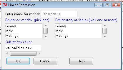
Figure 2. Screenshot linear regression menu. More than explanatory (predictor or independent) variables may be selected, but only one response (dependent) variable may be selected.
This procedure will handle simple and multiple regression problems. But before we go further, answer these two questions for the data set.
Question 1. What is the Response variable?
Question 2. What is the Explanatory variable?
Answers. See below in the R output to see if you were correct!
If there is only one predictor, then this is a Simple Linear Regression; if more than one predictor is entered, then this is a Multiple Linear Regression. We’ll get some more detail, but for now, identify and evaluate the test (p-value) of the slope coefficient (labeled after the name of the predictor variable), the test of the intercept coefficient, and some new stuff.
R output
RegModel.1 <- lm(Matings ~ Female, data=birds)
summary(RegModel.1)
Call: lm(formula = Matings ~ Female, data = birds)
Residuals:
     Min       1Q     Median         3Q        Max
-2.32805 -1.59407   -0.04359    1.77292    2.67195

Coefficients:
              Estimate    Std. Error     t value    Pr(>|t|)
(Intercept)    -8.6175        3.5323      -2.440     0.02528 *
Female          0.3670        0.1042       3.524     0.00243 **
---
Signif. codes: 0 '***' 0.001 '**' 0.01 '*' 0.05 '.' 0.1 ' ' 1
Residual standard error: 1.774 on 18 degrees of freedom
Multiple R-squared: 0.4082, Adjusted R-squared: 0.3753 F-statistic: 12.42 on 1 and 18 DF, p-value: 0.002427
In this example, slope = 0.367 and the intercept = -8.618. The first new term we encounter is called Multiple R-squared (R2) — it’s also called the coefficient of determination. It’s the ratio of the sum of squares due to the regression to the total sums of squares. R2 ranges from zero to 1, with a value of 1 indicating a perfect fit of the regression to the data.
Note 2. If you are looking for a link between correlation and simple linear regression, then here it is: R2 is the square of the product-moment correlation, r. Thus, r = √R2 see Chapter 17.2).
We introduced  in Chapter 17.1 . Interpretation of R2 goes like this: If R2 is close to zero, then the regression model does not explain much of the variation in the dependent variable; conversely, if R2 is close to one, then the regression model explains a lot of the variation in the dependent variable.
Did you get the Answers?
Answer 1: Number of matings
Answer 2: Size of females
Interpreting the output
Recall that
then

From the output we see that R2 was 0.408, which means that about 40% of the variation in numbers of matings may be explained by size of the females alone.
To complete the analysis get the ANOVA table for the regression.
Rcmdr: Models → Hypothesis tests → ANOVA table…
> Anova(RegModel.1, type="II")
Anova Table (Type II tests)
            Sum Sq   Df   F value      Pr(>F)
Female      39.084    1    12.415    0.002427 **
Residuals   56.666   18
---
Signif. codes: 0 '***' 0.001 '**' 0.01 '*' 0.05 '.' 0.1 ' ' 1
With only one predictor (explanatory) variable, note that the regression test in the ANOVA is the same (has the same probability vs. the null hypothesis) as the test of the slope.
Test two slopes
A more general test of the null hypothesis involving the slope might be
H0 : b1 = b vs. HA : b1 ≠ b
where b can be any value, including zero. Again, t-test would then be used to conduct the test of the slope, where the t-test would have the form

where SEb1-b2 is the standard error of the difference between the two regression coefficients. We saw something similar to this value back when we did a paired t-test. To obtain sb1–b2, we need the pooled residual mean square and the squared sums of the X values for each of our sample.
First, the pooled (hence the subscript p) residual mean square is calculated as

where resSS and resDF refer to residual sums of squares and residual degrees of freedom for the first (1) and second (2) regression equations.
Second, the standard error of the difference between regression coefficients (squared!!) is calculated as

where the subscript “1” and “2” refer to the X values from the first sample (eg, the body size values for the males) and the second sample (eg, the body size values for the females).
Note 3. To obtain the squared sum in R and Rcmdr, use the Calc function (eg, two sum the squared X values for the females, use SUM(‘Female’*’Female’)).
We can then use our t-test, with the degrees of freedom now

Alternatively, the t-test of two slopes can be written as
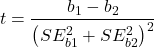
with again  .
In this way, we can see a way to test any two slopes for equality. This would be useful if we wanted to compare two samples (eg, males and females) and wanted to see if the regressions were the same (eg, metabolic rate covaried with body mass in the same way — that is, the slope of the relationship was the same). This situation arises frequently in biology. For example, we might want to know if male and female birds have different mean field metabolic rates, in which case we might be tempted to use a one-way ANOVA or t-test (since one factor with two levels). However, if males and females also differ for body size, then any differences we might see in metabolic rate could be due to differences in metabolic rate or to differences in the covariable body size. The test is generally referred to as the analysis of covariance (ANCOVA), which is the subject for Chapter 17.6. In brief, ANCOVA allows you to test for mean differences in traits like metabolic rate between two or more groups, but after first accounting for covariation due to another variable (eg, body size). However, ANCOVA makes the assumption that relationship between the covariable and the response variable is the same in the two groups. This is the same as saying that the regression slopes are the same. Let’s proceed to see how we can compare regression slopes, then move to a more general treatment in Chapter 17.6.
Example
For a sample of 13 tadpoles (Rana pipiens), hatched in the laboratory, oxygen consumption at rest was recorded with a YSI meter, model 51B, and a YSI oxygen – temperature probe (Yellow Spring Instruments Co., Yellow Springs, Ohio). Individual tadpoles were placed into a mason jar (volume 885 ml), with a magnetic stir bar housed in a slotted Petri dish glued to the bottom of the jar to gently stir the water. Water samples from the aquarium were used and petroleum jelly served as a sealant once the vessel had been fitted with the probe. Oxygen consumption was recorded in ppm and  values (ml O2 STP · hr-1). The tadpoles were scored for developmental stage by Gosner’s (1960) criteria. The tadpoles ranged from Gosner stage 35 to 44.
Note 4. Gosner stages 1 through 25 include the embryonic stages; By stage 31, toes develop on the limb buds; Following stage 40, substantial body changes are observed in the growing tadpole, transitioning from tailed tadpole to tail-less adult form. Complete metamorphosis is assigned Gosner stage 45.
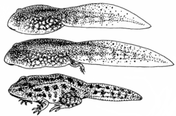
Figure 3. Pearson Scott Foresman, Public domain, via Wikimedia Commons

The question we addressed: metamorphosis of Anuran tadpoles to adults (frogs) likely involves increased metabolic demands, demands that may exceed simple allometric predictions based on increase in body size during development. Thus, we predicted that mass-specific metabolic rate for metamorphic frogs would exceed mass-specific metabolism of pre-metamorphic frogs.
M. Dohm unpublished results from my undergraduate days (1986!), you’ll find this simple data set at the bottom of this page (scroll or click here). For simplicity, we grouped all tadpoles between stages 35 and 38 as Stage I and all tadpoles between 39 and 44 as stage II. No tadpoles who completed metamorphosis were included in the dataset. It shouldn’t surprise you — with such a small sample size, the project lacked power to test the hypothesis, but many such studies, it’s worth looking at in the case anyway because the prevailing sentiment is that the metabolic cost of metamorphosis is significant — in other words, we expect a large effect size — and remains an ongoing research effort (see Burraco et al 2019).
You should confirm your self, but the slope of the regression equation of oxygen consumption (ml O2/hour) on body mass (g) was 444.95 (with SE = 65.89). Plot of data shown in Figure 4.
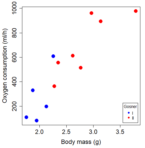
Figure 4. Scatterplot of oxygen consumption by tadpoles (blue: Gosner developmental stage I [35 – 38]; red: Gosner developmental stage II [39 – 44]), vs body mass (g).
The project looked at whether metabolism as measured by oxygen consumption was consistent across two developmental stages. Metamorphosis in frogs and other amphibians represents profound reorganization of the organism as the tadpole moves from water to air. Thus, we would predict some cost as evidenced by change in metabolism associated with later stages of development. Figure 5 shows a box plot of tadpole oxygen consumption by Gosner (1960) developmental stage.
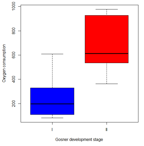
Figure 5. Boxplot of oxygen consumption by Gosner developmental stages (blue: stage I; red: stage 2).
Looking at Figure 4 we see a trend consistent with our prediction; developmental stage may be associated with increased metabolism. However, older tadpoles also tend to be larger, and the plot in Figure 4 does not account for that. Thus, body mass is a confounding variable in this example. There are several options for analysis here (eg, ANCOVA), but one way to view this is to compare the slopes for the two developmental stages. While this test does not compare the means, it does ask a related question: is there evidence of change in rate of oxygen consumption relative to body size between the two developmental stages? The assumption that the slopes are equal is a necessary step for conducting the ANCOVA, which we describe in Chapter 17.6.
So, divide the data set into two groups by developmental stage (12 tadpoles could be assigned to one of two developmental stages; one tadpole was at a lower Gosner stage than the others and so is dropped from the subset).
Gosner stage I (stages 35 – 39)
| Body mass | |
| 1.76 | 109.41 |
| 1.88 | 329.06 |
| 1.95 | 82.35 |
| 2.13 | 198 |
| 2.26 | 607.7 |
Gosner stage II (stage 40 – 44)
| Body mass | |
| 2.28 | 362.71 |
| 2.35 | 556.6 |
| 2.62 | 612.93 |
| 2.77 | 514.02 |
| 2.97 | 961.01 |
| 3.14 | 892.41 |
| 3.79 | 976.97 |
The slopes and standard errors were
| Gosner Stage I | Gosner stage II | |
| slope | 750.0 | 399.9 |
| standard error of slope | 444.6 | 111.2 |
Are the two slopes equal?
Looking at the table, we would say, no. slopes look different (750 vs 399.9). However, the errors are large and, given this is a small data set, we need to test statistically; are the slopes indistinguishable (Ho: bI = bII), where bI is the slope for the Gosner Stage I subset and bII is the slope for the Gosner Stage II subset?
To use our tests discussed above, we need sum of squared X values for Gosner Stage I and sum of squared for Gosner stage II results. We can get these from the ANOVA tables. Recall that after applying
ANOVA regression Gosner Stage I, R work
Anova(gosI.1, type="II")
Anova Table (Type II tests)

Response: VO2
            Sum Sq   Df    F value   Pr(>F)
Body.mass    89385    1     2.8461   0.1902
Residuals    94220    3
ANOVA regression Gosner Stage II
Anova(gosII.1, type="II")
Anova Table (Type II tests)

Response: VO2
             Sum Sq    Df   F value  Pr(>F)
Body.mass    258398     1    12.935  0.0156 *
Residuals     99882     5
Rcmdr: Models – Compare model coefficients..
compareCoefs(gosI.1, gosII.1)
Calls:
1: lm(formula = VO2 ~ Body.mass, data = gosI)
2: lm(formula = VO2 ~ Body.mass, data = gosII)

            Model 1    Model 2
(Intercept)   -1232       -441
SE              891        321

Body.mass       750        400
SE              445        111
SSgosnerI = 89385
SSgosnerII = 258398
We also need the residual Mean Squares (SSresid/DF resid) from the ANOVA tables
MSgosnerI = 94220/3 = 31406.67
MSgosnerII = 99882/5 = 19976.4
[under construction] Therefore, the pooled residual MS (s2x.y)p = nnn and the pooled SE of the difference sb1-b2 = nnn using the formulas above.
Now, we plug in the values I can get a t-test = (750 – 444.6)/nnn = nnn
The DF for this t-test are n1 + n2 – 4 = 4 + 6 – 4 = 6.
Using Table of Student’s t distribution (Appendix), I find the two-tailed critical value for t at alpha = 5% with DF = 6 is equal to 3.758. Since nn >> 3.758, we conclude that the two slopes are statistically different and P < 0.001 that the null hypothesis (Ho: bw = ball) was true. (edit: fix nn).
Questions
1. Write up three learning outcomes for this page. Hint: Point your favorite generative AI to this page and ask for help.
2. Metabolic rates like oxygen consumption over time are well-known examples of allometric relationships. That is, many biological variables (eg, is related as a · Mb, where M is body mass, b is scaling exponent (the slope!), and a is a constant (the intercept!)), and best evaluated on log-log scale. Redo the linear regression of oxygen consumption vs. body mass for the tadpoles, but this time, apply log10-transform to VO2 and to Body.mass. For example
Data in this page, bird matings
| Body.Mass | Matings |
|---|---|
| 29 | 0 |
| 29 | 2 |
| 29 | 4 |
| 32 | 4 |
| 32 | 2 |
| 35 | 6 |
| 36 | 3 |
| 38 | 3 |
| 38 | 5 |
| 38 | 8 |
| 40 | 6 |
Data in this page, Oxygen consumption, , of Anuran tadpoles
| Gosner | Body mass | VO2 |
|---|---|---|
| NA | 1.46 | 170.91 |
| I | 1.76 | 109.41 |
| I | 1.88 | 329.06 |
| I | 1.95 | 82.35 |
| I | 2.13 | 198 |
| II | 2.28 | 362.71 |
| I | 2.26 | 607.7 |
| II | 2.35 | 556.6 |
| II | 2.62 | 612.93 |
| II | 2.77 | 514.02 |
| II | 2.97 | 961.01 |
| II | 3.14 | 892.41 |
Gosner refers to Gosner (1960), who developed a criteria for judging metamorphosis staging.
Quiz Chapter 17.5
Testing regression coefficients
Chapter 17 contents
- Introduction
- Simple Linear Regression
- Relationship between the slope and the correlation
- Estimation of linear regression coefficients
- OLS, RMA, and smoothing functions
- Testing regression coefficients
- ANCOVA – Analysis of covariance
- Regression model fit
- Assumptions and model diagnostics for Simple Linear Regression
- References and suggested readings (Ch17 & 18)
9.4 – Heterogeneity chi-square tests
Planned comparisons and meta-analysis.
After finding evidence to reject the statistical null hypothesis, it may be appropriate to proceed to test a number of data sets against the same theoretical distribution. Provided these are planned comparisons, part of the experiment and not an exercise in data dredging (Norman 2014), you may proceed to test a series of nested models where groups are combined to make new groups for comparison. This approach is analogous to the post-hoc tests one may conduct after a statistically significant ANOVA (see Chapter 12.4) or when identifying a best-fit regression model (see Chapter 18.4).
Combining groups to make new comparisons — this scenario is consistent with a meta-analysis. A type of systematic review (Greenhalgh 1997, Akobeng 2005), meta-analysis is a statistical method that combines the results from multiple independent studies on the same topic to provide a more precise and robust overall conclusion. By combining studies, the goal is to calculate a pooled estimate as a measure of overall effectiveness of the treatment. Meta-analysis can increase the overall sample size, which improves the study’s ability to detect an effect if one exists. So, how to combine results from different studies ostensibly addressing the same hypothesis? Inevitably, some subjectivity will come into decisions about including or excluding studies — the goal is to identify quality studies, which may have conflicting conclusions and test whether a single conclusion of effectiveness is warranted based on a summary of evidence.
Here we introduce the Cochran’s Q test (Cochran 1954, Hoaglin 2016), aka a special case of the more general heterogeneity chi-square test. The null hypothesis is no significant difference in the proportion of “successes” across all groups being compared — any observed differences between the groups are just due to chance. The test statistic, Q, has a chi-square distribution with  degrees of freedom. A large Q value and small p-value suggest significant heterogeneity of results among the studies.
Note 1. As a reminder, “success” as an outcome category in epidemiology studies can represent any result depending on the study’s objective: survival, recovery, symptom improvement, or prevention of infection. The alternative outcome is generally referred to as “failure” (eg, death, non-recovery, no improvement, infection).
Heterogeneity tests ask whether results from combined studies are consistent; other tests exist, and are detailed in our special chapter on conducting meta-analysis. For example, I2 or I-squared test provides a measure of how much variation in the combined studies is due to true differences rather than by chance. In short, the I2 test quantifies how much — the percentage — the different studies agree, while the chi-square test returns a p-value that can be used to interpret whether that heterogeneity is statistically significant. We outline the basics of meta-analysis in Chapter 20.15. Other tests include DerSimonian-Laird test and Mandel-Paule test — these use the Q statistic and its distribution to estimate the between-study variance and provide better estimators with small sample size. Between-study variance is used to determine if a fixed-effect or a random-effects model (Chapter 12.3 and Chapter 14.3), is appropriate for the analysis. A random-effects model is used when significant heterogeneity is present (Higgins et al 2009).
Example.
Imagine a scenario where a population geneticist has collected allele (gene) frequency and genotype frequency data on single nucleotide polymorphisms (SNP) for the BRCA1 locus for three USA groups, African Americans, Asian Americans, and European Americans. Data of this kind can be obtained from the SNP database at NCBI (data retrieved 14 & 15 July 2014), and I collated several SNP involving a Cytosine base for Thymine base change (Table 1). The BRCA1 locus is on chromosome 17 and some of the hundreds of mutations found for this gene are associated with high risk of breast and or ovarian cancer (Couch and Weber 1996, Tram et al 2013).
Table 1. SNP of BRCA1 locus
| SNP | Population | n | C/C | C/T | T/T | C | T |
| rs1060915 | African American | 46 | 0.043 | 0.174 | 0,783 | 0.130 | 0.870 |
| Asian American | 48 | 0.083 | 0.625 | 0.375 | 0.396 | 0.604 | |
| European American | 48 | 0.167 | 0.458 | 0.375 | 0.396 | 0.604 | |
| rs3737559 | African American | 40 | 0.043 | 0.174 | 0.783 | 0.130 | 0.870 |
| Asian American | 48 | 0.083 | 0.625 | 0.292 | 0.396 | 0.604 | |
| European American | 48 | 0.167 | 0.458 | 0.375 | 0.396 | 0.604 | |
| rs799917 | African American | 124 | 0.048 | 0.258 | 0.694 | 0.177 | 0.823 |
| Asian American | 90 | 0.467 | 0.444 | 0.089 | 0.689 | 0.311 | |
| European American | 118 | 0.407 | 0.458 | 0.136 | 0.636 | 0.364 |
We may wish to test the combined data set to see if the large data set differs from Hardy Weinberg expectations before proceeding with a series of sample populations. By combining the data sets, we will be able to test whether one genotype is different from exception.
The goal then is to pool the data so that you have a more powerful test of the null hypothesis (remember our general discussion of statistical power and how increasing sample size increases your chances of correctly rejecting the null hypothesis).
For example, in our test of Hardy-Weinberg expectations (Example C), we calculated a  test of 7.8955. This test has k – 1 = 3 – 1 = 2 degrees of freedom. At alpha 5%, the critical value was 5.991 We clearly would reject the null hypothesis. But do we reject because of a difference in the aa, ab, or bb genotypes? Simply combine categories. Let’s test the homozygotes (aa and bb) versus the heterozygotes (ab).
Table 2. Worksheet
|
Categories
|
|||
| aa + bb | ab | n | |
|
Observed
|
66 | 34 | 100 |
|
Expected
|
52 | 48 | 100 |
 |
 |
||
With one degree of freedom, we clearly reject the null hypothesis because the critical value at 5% and one degree of freedom is equal to 3.841. To get the p-value, use
pchisq(7.852,df=1,lower.tail=FALSE)
which will return
[1] 0.005076452
Oh, and what was the null hypothesis? That there was an equal number of homozygotes and heterozygotes.
Other tests would be possible here, but the point is that you can dissect an experiment to determine which group is causing you to reject the null original hypothesis. While this is an important tool, you should also consider issues of apriori and aposterori decisions in experiments.
Questions.
1. The SNP rs1799971 (A > G) in the μ-opioid receptor (MOR) is associated with opioid dependency. Allele frequencies for different populations are provided in the table. Global frequency for A at this SNP is 0.188 (therefore frequency of G is 0.812).
| Population | n | A | G |
|---|---|---|---|
| African American | 32510 | 0.97 | 0.03 |
| Central American | 2450 | 0.81 | 0.19 |
| European | 18872 | 0.86 | 0.14 |
| Native American | 1260 | 0.86 | 0.14 |
| Native Hawaiian | 4534 | 0.75 | 0.25 |
| South Asian | 856 | 0.59 | 0.41 |
- Combine the data sets and test whether genotype frequency is different from the reported global exception.
- Test each population separately.
2. A behavioral ecologist studies the effect of three diets (high-protein, high-carbohydrate, and mixed) on the growth rate of juvenile frogs. Before collecting any data, she writes a protocol stating that she will compare only the high-protein vs mixed diet, based on a specific hypothesis about amino acid availability.
After analyzing the data, she also notices that frogs on the high-carbohydrate diet seem smaller, so she performs several additional pairwise comparisons that were not part of her original plan, reporting only the ones that are statistically significant.
Which statement best distinguishes the planned comparison from data dredging (p-hacking)?
A. The planned comparison is valid because it uses a larger sample size, while data dredging uses small samples.
B. The planned comparison was specified ahead of time based on a biological hypothesis, while data dredging involves unplanned tests added after seeing the data to search for significant results.
C. The planned comparison uses ANOVA, while data dredging uses regression.
D. The planned comparison must always produce a significant result, while data dredging never does.
Quiz Chapter 9.4
Heterogeneity chi-square tests
Chapter 9 contents
2.5 – Scientific method and where statistics fits
- Science isn’t just a recipe.
- Hypothetico-deductive reasoning.
- It’s all about the probability of a particular event.
- A statistical translation of the Scientific Method.
- When we say “experiment,” the hypothesis came first.
- Bottom-up, Top-down.
- How to interpret a test result.
- False discovery rate: claims must be stringently evaluated.
- Projects and the data lifecycle.
- Conclusions.
- Questions.
- Quiz.
- Chapter 2 contents .
Science isn’t just a recipe.
.
The scientific method is what makes science a “powerful way of knowing” (Church and Carpenter 2008), and by now, you should be familiar with the outline: hypothesis, experiment, etc. What distinguishes science from other fields of inquiry is that at its best, science accumulates verifiable evidence about our world. I begin with a disclaimer — our introductory textbooks tend to reify the scientific method (cf. Blachowicz 2009). Outside of the classroom and introductory science text books, I don’t think you’ll find much agreement among practicing scientists precisely what the scientific method entails, or whether strict adherence to a list of steps distinguishes what scientists do compared with other professions. For one difference, typical discussions of the scientific method may emphasize the experiment, which probably brings to mind images of a lab coat and test tubes, but should emphasize the critical thinking “tool kit” (Wivagg and Allchin 2002), eg, model-based inquiry. That said, holding a view that introductory textbooks should present nuances of epistemology seems a big ask.
But we do emphasize experimentation with good reason. In principle it is straightforward to identify what control groups are needed to conduct an experiment in the lab, but what are the control groups for an experiment conducted on the computer? In most cases, one should argue that if an outcome is obtained by random processes, then no additional cause need be addressed. Therefore, the control group for a simulation would be a random process generator.
Disagreements about the scientific method center about how science is really done (eg, from a social perspective), but also because there appear to be differences in approach in sciences that work on historical questions (physical cosmology, evolutionary biology, geology), and those that conform to the classic experimental approach (chemistry, molecular biology, physics). Epistemology is a fascinating area — How do we know what we know, What exactly is science and how is it different from other areas of knowing, etc. But I will leave you only with the tantalizing suggestion to read more and start with you with a list of readings to start (see Readings below). This is the stuff of graduate and professional school; we have work to do.
Despite apparent differences between what scientists say they do and how they actually do sciences, there is broad agreement; science as a way of knowing can be characterized by the following steps (National Academy of Sciences 1999).
- Begin with facts, which are observations confirmed and treated as true
- Formulate a hypothesis, with emphasis on hypotheses that are testable statements about relationships observed about the natural world
- Given the possible outcomes, state predictions derived from the hypothesis.
- Make observations of perform an experiment designed to test the hypothesis.
- Analyze the data from the experiment.
- Evaluate the results of the experiment against the predictions.
- Repeat.
This deceptively simple list hides much work to be done. Hypotheses are not “educated guesses,” where educated guess implies an idea about some phenomenon is likely the correct explanation because of the skill or knowledge of the person making the guess. Good hypotheses make possible experimental tests whose results can be used to rule out alternative explanations, sensu Platt’s “strong-inference”.
Hypothetico-deductive reasoning.
.
I mention this disclaimer about the common (and reassuring) textbook discourse on the scientific method to suggest that, if you have not already reached this point in your career, it is time to move past the cookbook approach to thinking about what it means to do science in practice. Yet another helpful reading is from a paper in Environmental Health by Ozonoff amd Grandjean (2020).
In other words, what makes “good science”?
There is induction and deduction and probabilistic thinking that must be grappled with, all emphasizing efforts by the individual, and yet science, if it is to make any progress must ultimately be a communal activity (Varmus 2009). In particular, to the extent a researcher consistently applies hypothetico-deductive reasoning, or as Platt (1964) called it, “strong-inference,” then good science can happen (see Fudge 2014 for an update). Strong inference according to Platt implies that researchers should follow three steps (after Fudge 2014):
- develop alternative hypotheses
- think of a crucial experiment that can exclude one or more hypotheses
- perform the experiment and obtain a clean result.
Then, beginning with step 1, repeat the procedure to refine the possibilities that remain.
The list of elements of the scientific method neglected to address the crucial role of scientists engaged in an active community of scientists fits in. However, we can can quickly suppose that every step of the scientific method can involve input from others to help shape, improve, and indeed carry out the activities needed to practice science. What scientists share is critical thinking and the tools of statistics provides a common language.
It’s all about the probability of a particular event.
.
Platt (1964) wrote that the observations we make that are puzzling or hard to explain, which implies our understanding is incomplete. We then proceed to ask questions about why the observations are different from our expectations, and we speculate about how the outcome comes about. Thus, we have to consider the probability, or chance, of a particular outcome (event) compare to other possible outcomes. Statistics is about analyzing the probability of outcomes. But there is a twist; there are two distinct, but complementary approaches to statistics. Most of the statistics you have been taught so far comes from the frequentist approach. That is, how often (frequency) will we get the kind of results we observe given the hypothesis? Another approach can be termed Bayesian, where the question is how likely is the hypothesis to be correct given the data? These two approaches view the data obtained from the same experiment differently. A frequentist views the data as random — repeat the experiment and the results will differ — but the hypothesis is fixed (it is either true or it is not). A Bayesian on the other hand views the hypothesis as random with a probability of being true somewhere between zero and 100 percent and the data are fixed.
Which are you, a frequentist, or a Bayesian? Consider the following from xkcd.com no. 1132 (Fig. 1).
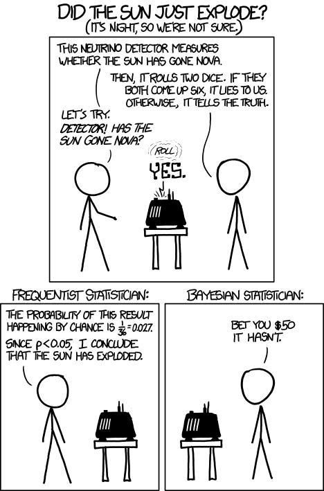
Figure 1. “Frequentists vs Bayesians,” xkcd.com no. 1132
The Bayesian approach makes sense when there exists prior knowledge — the Sun came up this morning, as it did the day before, and the day before that, etc. New data are assessed against what we already know. The Frequentist approach, despite philosophical shortcomings, works for analyzing experiments where prior knowledge is lacking about outcomes. Because much of biomedical research is based on the Frequentist approach, most of our efforts, too, will utilize that approach.
A statistical translation of the Scientific Method.
.
Given our frequentist perspective, we can outline our Scientific Method as follows.
- Formulate a Null and an Alternative hypothesis.
- State predictions from the Null and an Alternative hypotheses.
- Design an experiment or observation.
- Analyze the data from the experiment or observation.
- Interpret the experiment or observation.
- Evaluate the predictions from the Null and an Alternative hypotheses.
- Accept (provisionally) or reject (provisionally) the Null hypothesis.
- Evaluate model fit and robustness
- Repeat.
In practice, there is more to statistics than these 8(9) steps, but this does provide the outline of what statistical analyses are about. There are nuances to how a Frequentist or a Bayesian views statistical analyses as evidence for or against a conclusion (Goodman 1999a, 1999b). We need to distinguish between when data are acquired in the process; data may come before or after the hypotheses are stated. In epistemology, hypotheses are either a priori or a posterori and we need to add these to our discussion of Scientific Method. The terms are Latin, translated apparently as “from the earlier” and “from the later, respectfully.
Note from the lists described as “the” scientific method how hypothesis comes first. Folks who think and write about how and why we know what we know — the discipline is called epistemology — tell us we are generally on more solid footing when we design experiments with specific intent, specific and testable hypotheses. The branch of statistics concerned with experimental design provides rich context for many practical aspects of how to implement experiments — in other words, how to follow the Scientific Method, even if turns out there isn’t just one universal definition of Scientific Methods out there.
When we say “experiment,” the hypothesis came first.
.
More commonly in statistics, the phrases planned, and therefore a priori, and unplanned or a posterori, comparisons are referenced. In practice, biologists design experiments and make observations accordingly to test one or more hypotheses, but they may also address additional hypotheses after the fact. Especially if the experiment generates a lot of data.
You may have also heard of the phrase data mining. Data mining is loosely defined, but mostly refers to sets of protocols and procedures to extract patterns from large data sets stored in databases. Google apparently does lots of data mining as do many other businesses that obtain large amounts of data. Unplanned comparisons includes any data mining protocols, no matter how sophisticated the language sounds (feature selection, classification tree). Data mining is not consistent with classic experiments; it’s different than Step 6 (Step 8 in the second list) listed above because no new data or experiment is carried out.
Can you get away with coming up with and testing new hypotheses from data gathered from an experiment designed to test a different hypothesis? Yes, and of course, the process can be quite profitable for Google. However, you should proceed with caution and restraint. If you are not careful about how you write it up — you will probably be called on it by a reviewer of your work. Is this a posterori approach still science? Of course, yes! I’d even go so far as to say that when one studies real systems, you can’t limit yourself to only planned hypotheses and testing. At least, one designs experiments and carries out those tests but then also uses current data to generate new ideas. Science is also exploratory — you may not design an experiment at all, but through observations, you probably will develop testable hypotheses! We’ll return to these concepts soon. What you must be aware of in any unplanned comparison or data mining sojourn is the possibility of committing a data dredging (aka p-hacking) sin — searching through data to come up with misleading, but statistically “significant” results (Ioannidis 2007; Stefan and Schönbrodt 2023).
Testing of unplanned a posterori hypotheses is a real concern in science. On the one hand, those who think about how we learn about the world and make sense of it have stated emphatically that the best way we know is to follow the scientific method — and that begins with hypotheses followed by designed experiments to test claims derived from those a priori hypotheses. We (teachers, textbook author) continue to teach science as the act of individuals toiling away in the forest or in the lab, pursuing sets of questions that may involve the collection of measurements on dozens to a few hundred subjects. While this type of science is still in practice, there is no doubt that big science involving many people is more common and, perhaps, better at generating new knowledge (Wuchty et al 2007). One result of “big science” is to generate a lot of data, the very essence now of big data, and there must be room for testing of new hypotheses gathered on data sets. This is the essence of the argument for the ENCODE project (ENCODE Project Consortium 2012) — generate lots of genetic data on the human genome using common techniques and make the data publicly available — new research can be conducted on old data.
Bottom-up, top-down.
.
Consider the pronouncements (almost daily it seems!) about the discovery of a new gene for some disease, process, or behavior in humans. Often times, although not always, these “discoveries” are not duplicated by other research groups. Why not? Well, for one, the phrase “gene for” is a dubious shorthand for what is usually a more complex causation. But from our statistical perspective it is problematic because the search for genes is really an a posterori exercise — one begins with phenotypic differences (some have the disease, others do not) and some genetic information (SNPs, DNA sequencing) and then proceeds to see if there are any differences in the genetic material at hand between the two groups. This approach, the Genome Wide Association Study, or GWAS, would be termed “top-down” — begin with the phenotypic differences and search for genetic differences between those that do and those who do not have the condition. Sampling is an issue (are the unaffected subjects a random sample from the entire population?), but the problem also is one of logical design — the hypothesis is made after the fact — a statistical difference between the groups is attributed to a particular genetic difference.
Case-control subjects, where patients with the condition are matched with other individuals who do not have the condition, but match in other ways (eg, age, income, etc.), are enrolled in such studies because there can be no random assignment of subjects to treatment. Case-control subjects are selected such that affected and unaffected individuals are matched by characteristics in as many meaningful ways as possible (eg, age, gender, income, etc.). Because many tests are conducted in GWAS studies, ie, is there a difference between the control and affected group for the first gene, the second gene, and so on up to the number of genes on the microarray chip (10,000 or more genes), the chance that any particular association is a false positive is high, discussed further when we cover Risk Analysis in Chapter 7.
How to interpret a test result.
You are a medical doctor reading the results of a test for three-month average glycated hemoglobin, A1C, levels for your patient. For example, A1C above 6% is considered strong marker of diabetes. A marker, yes, but not the same as a guarantee that a person has diabetes. A false positive (FP) is the case where a test result is positive, but the subject in fact does not have the condition. False positive is equal to the ratio of

where FP is number of false positive readings and TN refers to the true negative, those who in fact do not have the condition.
In Chapter 7 we will spend some time on risk analysis. To introduce this important subject in biostatistics, we’ll begin with an example. A study of 15,934 subjects without diagnosed diabetes found 3.8% or 605 individuals had elevated A1C levels, or about 7.1 million adults not yet diagnosed with diabetes (Selvin et al 2011). About 90% of these individuals also had fasting glucose levels greater than 100 mg/dL, i., diabetic. This is clearly a good test. However, note that 10% of the 605 individuals had elevated A1C, but fasting glucose levels less than 100 mg/dl, ie, did not meet the diagnostic of type 2 diabetes. Thus, the false positive rate is about 0.4%, or nearly 30,000 adults with elevated A1C without diabetes.
Working through frequencies can be challenging, so applying a natural number approach helps. Having just read through the frequencies and percentages, now look at how they translate to probability tree (Fig. 2). Start by utilizing a per capita rate standard: for proportions in the 10 – 20% range, a standard 1000 persons works well (Fig. 2).
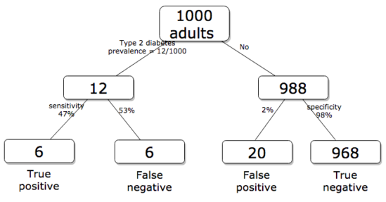
Figure 2. Probability tree diagram with prevalence of type 2 diabetes and sensitivity, specificity of A1C test, data from CDC and Selvin et al 2011. Tree drawn with free diagrams.net app.
How many expected to have A1C above 6%? Twenty-six total positives, only 23% are true positives. An important lesson is that if the prevalence of a condition is low, then any diagnostic test with high sensitivity necessarily will identify many false positives.
False discovery rate: claims must be stringently evaluated.
.
The genome scientists involved in GWAS studies generally are aware of false positives, also termed false discovery rate (FDR), conduct statistical corrections to account for false positives (eg, Brzyski et al 2016), and generally are cautious in their interpretation. But not always. Studies of associations between autism and environment come to mind (eg, Waldman et al 2008), and recent developments in the direct-to-consumer genetic testing market also suggest that the limitations of these kinds of studies are not always represented.
There is a broader concern about the reliability of research, and the debate about how to improve reliability comes from a call to understand how to do statistics better and, more importantly to understand how statistics are to be used in making claims from statistical results (Ioannidis 2007; but see Goodman and Greenland 2007). A key element of scientific work is that findings are repeatable: results from one group should apply to other groups. One dictate to improve reproducibility — increase number of subjects in studies — is obvious, but given the cost of GWAS, currently an unreasonable demand.
In some cases, biologists already have a particular gene in mind, whose function is more or less known, and then the exercise follows the Scientific Method listing much more directly. This bottom-up approach leads to a straightforward, testable genetic hypotheses: a specific difference in genomic sequence predicts a difference in phenotype outcome. A good example is the identification of more than 100 different single nucleotide mutations, called single nucleotide polymorphisms or SNPs, in the CFTR gene of patients known to have cystic fibrosis disease (Castellani 2013). As of August 2018, the number of known pathogenic or likely pathogenic SNPs is now listed at 440 in the SNP database; to put this in some context, there are more than 40,000 reported single nucleotide polymorphisms for the CFTR gene (this number includes SNP duplicates).
Projects and the data lifecycle.
A requirement for our biostatistics course, students are asked to design and implement a research project during the semester (Hydorn 2019). The project can either be part of an ongoing student research project or solely confined to the biostatistics course. The topics are diverse, ranging from observational to experimental to systematic reviews from the disciplines of biology, environmental science, and public health. Examples of project ideas implemented in the biostatistics and related courses at Chaminade University include:
- effects of environmental stress on growth rates.
- 2D and 3D shape analysis of mollusk shells.
- Individual variation and fluctuating asymmetry of plant leaves and flowers along an altitudinal gradient
- several systematic reviews (meta analysis) of published works of interest to public health
- vaccination benefits and risks.
- pain management of over the counter vs prescription medication.
- efficacy of “alternative medicine” approaches to health.
- comparisons of types of medical insurance on patient outcomes of knee replacement therapy.
The justification for the project learning activity is that it provides hands-on opportunity to apply statistical and data sciences concepts to real-world problems. Students work through the challenges of developing a research question, identifying testable hypotheses, designing a study, collecting data, performing analysis, and interpreting results. Importantly, students must decide for themselves which statistical tests and methods are most appropriate for their unique data, rather than simply following a formula presented in a lecture. This connects abstract statistical ideas to practical application, promoting a deeper, more lasting understanding. We manage the projects by encouraging a research lab community: students discuss with their peers their ideas, their data collection and experimental design challenges, with the instructor serving to guide and mentor the multiple projects and intervene as needed to steer student projects towards completion.
Throughout the semester we model the project approach. Students are encouraged to create a working folder on their computer, while dividing homework and other assignments into named projects. Students are also asked to address aspects of their project’s data life cycle (Borgman 2019, Ezer and Whitacker 2019, Griffin et al 2018). A quick Google search on the phrase returns millions of hits (see Note 1), but key elements of the concept are that projects have a beginning and an end, and it is helpful — and in the case of our statistics course, required — to address project management.
Note 1: For example, “8 Steps in the Data Life Cycle,” by Tim Tobierski of Harvard Business School.
BI-311 students, see Homework 1: Project data life cycle in Mike’s Workbook for Biostatistics.
Projects include data generation and collection, data processing, storage and data management, data exploration and visualization, interpretation and reporting. Thus, students need to develop a data management plan, which includes how data are collected, application of best practices to insure data file and storage of images, and how to share the project results. We ask students to develop 10-min research talks, which are presented and recorded, suitable for ePortfolio inclusion.
Conclusions.
.
Epistemology, the theory of how knowledge is acquired, is a complicated business – what I want you to appreciate now is that planned and unplanned comparisons affect interpretation of your statistical results, how the difference is likely also to affect the reproducibility of your work. In the language or clinical trials and experimental design, planned and unplanned accompany prospective and retrospective studies (Chapter 5). A prospective study in the case of GWAS means genetic differences among individuals are known at the start of the study, and phenotypic differences arise naturally during the course of the study. Knowing the strengths and limitations of, for example, a planned retrospective study is at the heart of experimental design (Chapter 5).
In the biostatistics course, students are required to design and carry out an independent research project that integrates statistical methods with real-world problems in biology, environmental science, or public health. The course emphasizes hands-on learning through the full research process—from formulating questions to data collection, analysis, and interpretation—while fostering a collaborative research lab environment. Students also learn project and data management skills and conclude by presenting their findings in recorded research talks suitable for inclusion in an ePortfolio.
Questions.
- Write up three learning outcomes for this page. Hint: Point your favorite generative AI to this page and ask for help.
- Above we described how GWAS studies are generally top-down; What would constitute a bottom-up approach to GWAS?
- In your own words provide pro and con points of view on data mining of large data sets.
- Create a stylized infographic, like a mind map, to illustrate the data life cycle for a one semester research project.
Quiz Chapter 2.5
Scientific method and where statistics fits
Chapter 2 contents
.