16.3 – Data aggregation and correlation
Introduction
Correlations are easy to calculate, but interpretation beyond a strict statistical interpretation, eg, two variables linearly associated, may be complicated — caution is recommended. With respect to interpreting a correlation, caution and temperance is warranted. As previously discussed, “correlation is not causation,” is well known, but identifying when this applies to a particular analysis is not straight-forward. We introduced the problem of two variables sharing a hidden covariation which drives the correlation. In this section we introduce how correlations among grouped (aggregated) data may be quite different from the underlining individual correlations (cf Robertson 1950, Greenland 2001, Portnov et. al 2006).
Perfect (+1 or -1) correlation?
What if an estimated correlation value between two ratio scale variables turns out to be +1 or -1, the limits of the possible range of the correlation coefficient? Trivially, the reported value of one for the coefficient may be the result of rounding, it was actually 0.97. But, for argument’s sake, let’s assume the coefficient value was 1.0 to as many significant figures as the calculator may report. Another trivial possibility: suspect you’re looking at a case for which the two variables are the same thing, but on different scale. For example, the correlation between a range of temperatures measured in degrees Fahrenheit and then converted to degrees Celsius trivially will be +1.
Less trivially, a correlation of +1 or -1 may reveal that two variables are simply restatements of the same measured variable. Additionally, perfect correlation may reflect construction of a composite variable. Composite variables are examples of indexes, and are constructed from related variables by the researcher in order to better predict multivariate outcomes (see also Latent variables). Refs to add Diamantopoulos and Winklhofer 2001; Bollen and Diamantopoulos 2015
Data aggregation
Data aggregation or grouping refers to processes to group data in a summary form. Considerable public health data is presented this way. For example, CDC reports table after table of data about morbidity and mortality of United States of America population. Data are grouped by age, cities, counties, ethnicities, gender, and states and reports are generated to convey the status of health peoples. Similarly, education statistics, economic statistics, and statistics about crime are commonly crafted from grouped data of what originally was data for individuals.
Correlations between groups may yield spurious conclusions
Researchers interested in testing hypotheses like BMI is correlated with mortality (Flegal et al 2013, Kltasky et al 2017), or health disparities and ethnicity (Portnov et. al 2006), may use grouped data. In 16.2 we introduced the concept of spurious correlation. Correlations between grouped data may also mislead.
Consider the hypothesis that religiosity may deter criminal behavior. This hypothesis has been tested many times dating back to at least the 1940s (reviewed in Salvatore and Rubin 2018). Conclusions about religious beliefs range from negative association with criminal behavior to, in some reports, holding religious beliefs makes one more likely to commit crime. Testing versions of the hypothesis — what causes criminality in some individuals — among a variety of putative causal agents pops up through the history of biology research, arguably beginning with Galton. I hope you appreciate how challenging this would be to actually resolve — defining criminal behavior itself is laden with all kinds of sociology traps — and for a biologist, reeks of eugenics lore (Horgan 1993).
that all said, let’s proceed to test the religion-criminality hypothesis with aggregated data. The null hypothesis would be no association between crime statistics and numbers of churches. We can also ask about association between crime and non-religious or secular beliefs. I added numbers of Catholic churches and secular humanists groups for cities larger than 100K population by Internet search (FBI for crime statistics, Wikipedia for cities). Figure 1 and Figure 2 report crimes statistics aggregated by cities in the United States and by number of Catholic churches (Fig 1), and by number of secular humanists groups (Fig 2) in the same cities.
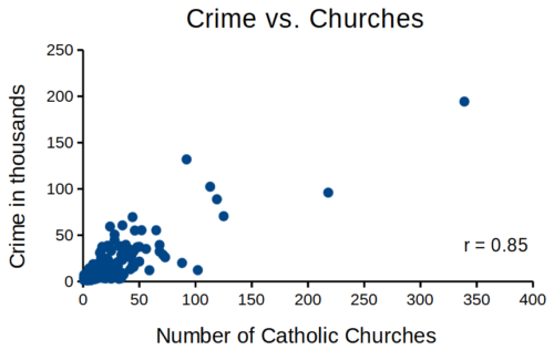
Figure 1. Scatterplot crime rates of cities by number of Catholic churches
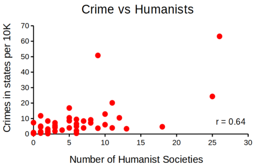
Figure 2. scatterplot crime rates of cities by number of secular humanist associations.
We’ll just take the numbers on faith (of course, we should think about the bunching around the origin — do we really think Internet search will get all of the secular groups, for example? Or is it really the case that several cities have no secular groups?). Both correlations were statistically different from zero, crime by churches (P < 0.001) and crime by secular groups (P < 0.001).
Now, having read Chapter 16.2 I trust you recognize immediately that there’s an important hidden covariate in common. Cities with small populations will have small numbers of crimes reported and smaller numbers of churches compared to large cities. Indeed, the correlation between population and crime for these cities was 0.89 and 0.97, respectively. However, after estimating the partial-correlations, we still have some explaining to do. For crime and churches, the partial correlation was +0.37 (p-value = 0.009); for crime and secular humanist groups, the partial correlation was -0.37 (p = 0.018). These results suggest that persons are more likely to commit crimes in cities with lots of Catholic churches whereas criminal behavior by individuals is less likely where secular humanist groups are numerous.
Before we start pointing fingers, the analysis presented here is a classic ecological fallacy. By grouping the data we lose information about the individuals, and it is the individuals to which the hypothesis applied. Thus, we are at risk of making incorrect conclusions by assuming that the individual is characterized by the group. The hypothesis remains challenging to test (how does one get a valid assessment of an individual’s religiosity? The hypothesis is challenging to test, but studies of individuals tend to find no association or a negative association between criminal behavior and religiosity (Salvatore and Rubin 2018). Crime statistics may underestimate criminal behavior, eg, embezzlement and other “white” crime), but a proper study would look to survey of individuals (Fig 3).
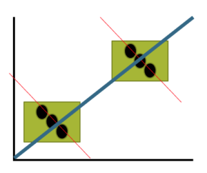
Figure 3. Illustration of ecological fallacy: positive association at level of groups (boxes, solid blue line), but negative association at level of individuals (black circles, red dashed lines).
Studies that use aggregate data test hypotheses about the groups, not about individuals in the groups. These studies are appropriate for comparing groups, eg, health disparities by ethnicity (Wang Kong et al 2022) or gender (Read and Gorman 2010; Cooper et al 2023), or comparisons among counties (eg, urban vs. rural) for medical resources (Anderson and Zimmerman 2024), or other “social determinates of health” (Crawfolrd 1977; Braveman and Gottlieb 2014), but one cannot conclude that the association is present for members of the group.
Bubble charts
Given we know about the covariation with population size, is there a better way to visualize the crime by number of churches and crime by number of humanist societies? One option is the bubble chart.
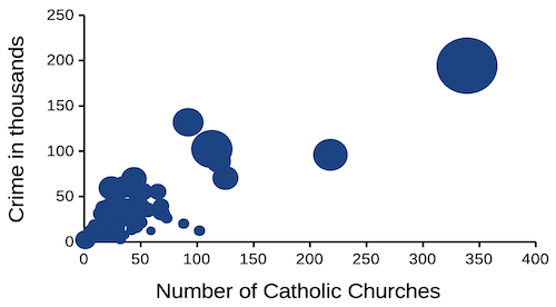
Figure 4. Bubble plot of data used to make Figure 1. Plot by LibreOffice Calc.
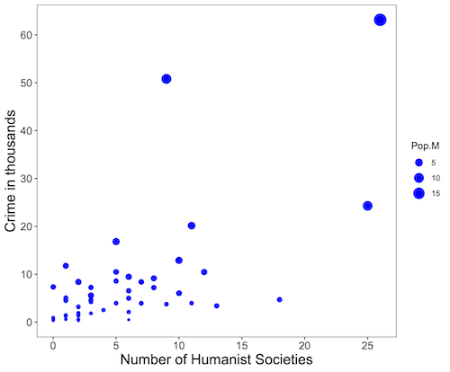
Figure 5. Bubble plot of data used to make Figure 2. Plot by ggplot2 package in R.
R code for Figure 5.
# STDHA site by Dr A. Kassambara https://www.sthda.com/english/

myPlot <- ggplot(humanists, aes(x = Humanist, y = Crime.K, size = Pop.M)) +
geom_point(color="blue", aes(size = Pop.M)) + theme_bw() + ylab("Crime in thousands") +
xlab("Number of Humanist Societies")

myPlot2 <- myPlot + theme(axis.title=element_text(size=16),
axis.text.x=element_text(size=12), axis.text.y=element_text(size=12),
panel.grid.major = element_blank(), panel.grid.minor = element_blank())

myPlot2 + scale_x_continuous(breaks=seq(0,30,5)) +
scale_y_continuous(breaks=seq(0,65,10))
Questions
1. Write up three learning outcomes for this page. Hint: Point your favorite generative AI to this page and ask for help.
2. What’s the most likely statistical explanation for why there is an apparent correlation between rates of autism and childhood vaccination rates? See Davidson 2017.
3. For the following data set, calculate the Pearson product moment correlation and, separately, the Spearman rank correlation. Report the values of the coefficients and provide an interpretation of the results.
v1: 68, 72, 68, 69, 65, 76, 58, 62, 69, 67, 66, 71, 70
v2: 1.727, 1.829, 1.727, 1.753, 1.651, 1.93, 1.473, 1.575, 1.753, 1.702, 1.676, 1.803, 1.778
4. For a small data set on human males ages 24 to 59, the estimated correlation between weight and the calculated BMI index was 0.68. (BMI is an example of a composite variable.) Explain why the correlation between weight and BMI is not +1.
Quiz Chapter 16.3
Data aggregation and correlation
Chapter 16 contents
16.2 – Causation and Partial correlation
Introduction
Science driven by statistical inference and model building is largely motivated by the the drive to identify pathways of cause and effect linking events and phenomena observed all around us. (We first defined cause and effect in Chapter 2.4) The history of philosophy, from the works of Ancient Greece, China, Middle East and so on is rich in the language of cause and effect. From these traditions we have a number of ways to think of cause and effect, but for us it will be enough to review the logical distinction among three kinds of cause-effect associations:
- Necessary cause
- Sufficient cause
- Contributory cause
Here’s how the logic works. If A is a necessary cause of B, then the mere fact that B is present implies that A must also be present. However, that the presence of A does not imply that B will occur. If A is a sufficient cause of B, then the presence of A necessarily implies the presence of B. However, another cause C may alternatively cause B. Enter the contributory or related cause: A cause may be contributory if the presumed cause A (1) occurs before the effect B, and (2) changing A also changes B. A contributory cause does not need to be necessary nor must it be sufficient; contributory causes play a role in cause and effect.
Thus, following this long tradition of thinking about causality we have the mantra, “Correlation does not imply causation.” The exact phrase was written as early as emphasized by Karl Pearson who invented the statistic back in the late 1800s. This well-worn slogan deserves to be on T-shirts and bumper stickers*, and perhaps to be viewed as the single most important concept you can take from a course in philosophy/statistics. But in practice, we will always be tempted to stray from this guidance. The developments in genome-wide-association studies, or GWAS, are designed to look for correlations, as evidenced by statistical linkage analysis, between variation at one DNA base pair and presence/absence of disease or condition in humans and animal models. These are costly studies to do and in the end, the results are just that, evidence of associations (correlations), not proof of genetic cause and effect. We are less likely to be swayed by a correlation that is weak, but what about correlations that are large, even close to one? Is not the implication of high, statistically significant correlation evidence of causation? No, necessary, but not sufficient.
Note 1. A helpful review on causation in epidemiology is available from Parascandola and Weed (2001); see also Kleinberg and Hripcsak (2011). For more on “correlation does not imply causation”, try the Wikipedia entry. Obviously, researchers who engage in genome wide association studies are aware of these issues: see for example discussion by Hu et al (2018) on causal inference and GWAS.
Causal inference (Pearl 2009; Pearl and Mackenzie 2018), in brief, employs a model to explain the association between dependent and multiple, likely interrelated candidate causal variable, which is then subject to testing — is the model stable when the predictor variables are manipulated, when additional connections are considered (eg, predictor variable 1 covaries with one or more other predictor variables in the model). Wright’s path analysis, now included as one approach to Structural Equation Modeling, is used to relate equations (models) of variation in observed variables attributed to direct and indirect effects from predictor variables.
* And yes, a quick Google search reveals lots of bumper stickers and T-shirts available with the causation  sentiment.
Spurious correlations
Correlation estimates should be viewed as hypotheses in the scientific sense of the meaning of hypotheses for putative cause-effect pairings. To drive the point home, explore the web site “Spurious Correlations” at https://www.tylervigen.com/spurious-correlations , which allows you to generate X-Y plots and estimate correlations among many different variables. Some of my favorite correlations from “Spurious Correlations” include (Table 1):
Table 1. Spurious correlations, https://www.tylervigen.com/spurious-correlations
| First variable | Second variable | Correlation |
| Divorce rate in Maine, USA | Per capita USA consumption of margarine | +0.993 |
| Honey producing bee colonies USA | Juvenile arrests for marijuana possession | -0.933 |
| Per capita USA consumption of mozzarella cheese | Civil engineering PhD awarded USA | +0.959 |
| Total number of ABA lawyers USA | Cost of red delicious apples | +0.879 |
These are some pretty strong correlations (cf. effect size discussion, Ch11.4 and 16.1), about as close to +1 as you can get. But really, do you think the amount of cheese that is consumed in the USA has anything to do with the number of PhD degrees awarded in engineering or that apple prices are largely set by the number of lawyers in the USA? Cause and effect implies there must also be some plausible mechanism, not just a strong correlation.
But that does NOT ALSO mean that a high correlation is meaningless. The primary reason a correlation cannot tell about causation is because of the problem (potentially) of an UNMEASURED variable (a confounding variable) being the real driving force (Fig 1).
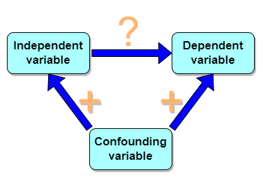
Figure 1. Unmeasured confounding variables influence association between independent and dependent variables, the characters or traits we are interested in.
Here’s a plot of running times for the best, fastest men and women runners for the 100-meter sprint. Running times over 100 meters of top athletes since the 1920s. The data are collated for you and presented at end of this page (scroll or click here).
Here’s a scatterplot (Fig 2).
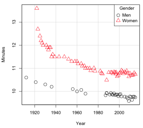
Figure 2. Running times over 100 meters of top athletes since the 1920s.
There’s clearly a negative correlation between years and running times. Is the rate of improvement in running times the same for men and women? Is the improvement linear? What, if any, are the possible confounding variables? Height? weight? Biomechanical differences? Society? Training? Genetics? … Performance enhancing drugs…?
If we measure potential confounding factors, we may be able to determine the strength of correlation between two variables that share variation with a third variable.
The partial correlation
There are several ways to work this problem. The partial correlation is a useful way to handle this problem, i.e., where a measured third variable is positively correlated with the two variable you are interested in.

Without formal mathematical proof presented, r12.3 is the correlation between variables 1 and 2 INDEPENDENT of any covariation with variable 3.
For our running data set, we have the correlation between women’s time for 100m over 9 decades, (r13 = -0.876), between men’s time for 100m over 9 decades (r23 = -0.952), and finally, the correlation we’re interested in, whether men’s and women’s times are correlated (r12 = +0.71). When we use the partial correlation, however, I get r12.3 = -0.819… much less than 0 and significantly different from zero. In other words, men’s and women’s times are not positively correlated independent of the correlation both share with the passage of time (decades)! The interpretation is that men are getting faster at a rate faster than women.
In conclusion, keep your head about you when you are doing analyses. You may not have the skills or knowledge to handle some problems (partial correlation), but you can think simply — why are two variables correlated? One causes the other to increase (or decrease) OR the two are both correlated with another variable.
Testing the partial correlation
Like our simple correlation, the partial correlation may be tested by a t-test, although modified to account for the number of pairwise correlations (Wetzels and Wagenmakers 2012). The equation for the t test statistic is now
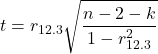
with k equal to the number of pairwise correlations and n – 2 – k degrees of freedom.
Examples
Lead exposure and low birth weigh. The data set is numbers of low birth weight births (< 2,500 g regardless of gestational age) and numbers of children with high levels of lead (10 or more micrograms of lead in a deciliter of blood) measured from their blood. Data used for 42 cities and towns of Rhode Island, United States of America (data at end of this page, scroll or click here to access the data).
A scatterplot of number of children with high lead is shown below (Fig 3).
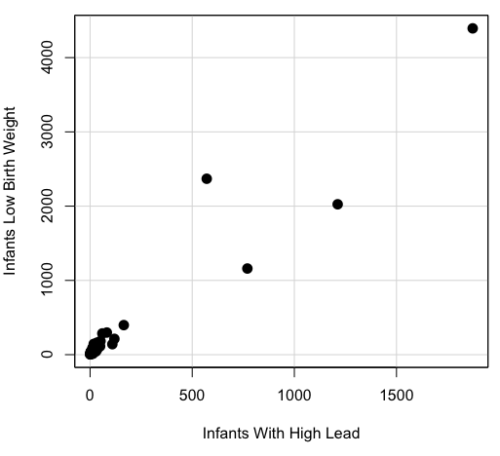
Figure 3. Scatterplot birth weight by lead exposure.
The product moment correlation was r = 0.961, t = 21.862, df = 40, p < 2.2e-16. So, at first blush looking at the scatterplot and the correlation coefficient, we conclude that there is a significant relationship between lead and low birth weight, right?
However, by the description of the data you should recall that counts were reported, not rates (eg, per 100,000 people). Clearly, population size varies among the cities and towns of Rhode Island. West Greenwich had 5085 people whereas Providence had 173,618. We should suspect that there is also a positive correlation between number of children born with low birth weight and numbers of children with high levels of lead. Indeed there are.
Correlation between Low Birth Weight and Population, r = 0.982
Correlation between High Lead levels and Population, r = 0.891
The question becomes, after removing the covariation with population size is there a linear association between high lead and low birth weight? One option is to calculate the partial correlation. To get partial correlations in Rcmdr, select
Statistics → Summaries → Correlation matrix
then select “partial” and select all three variables (select + Ctrl key; (Windows or macOS) (Fig 4).
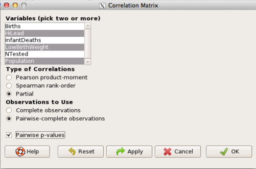
Figure 4. Screenshot Rcmdr partial correlation menu
Results are shown below.
partial.cor(leadBirthWeight[,c("HiLead","LowBirthWeight","Population")], tests=TRUE, use="complete")

Partial correlations:
                 HiLead LowBirthWeight Population
HiLead          0.00000        0.99181   -0.97804
LowBirthWeight  0.99181        0.00000    0.99616
Population     -0.97804        0.99616    0.00000
Thus, after removing the covariation we conclude there is indeed a strong correlation between lead and low birth weights.
Note 2. Some verbiage about correlation tables (matrices). The matrix is symmetric and the information is repeated. I highlighted the diagonal in green. The upper triangle (red) is identical to the lower triangle (blue). When you publish such matrices, don’t publish both the upper and lower triangles; it’s also not necessary to publish the on-diagonal numbers, which are generally not of interest. Thus, the publishable matrix would be
Partial correlations:
                LowBirthWeight Population
HiLead                 0.99181   -0.97804
LowBirthWeight                    0.99616
Another example
Do Democrats prefer cats? The question I was interested in, Do liberals really prefer cats, was inspired by a Time magazine 18 February 2014 article. I collated data on a separate but related question: Do states with more registered Democrats have more cat owners? The data set was compiled from three sources: 2010 USA Census, a 2011 Gallup poll about religious preferences, and from a data book on survey results of USA pet owners (data at end of this page, scroll or click here to access the data).
Note 3: This type of data set involves questions about groups, not individuals. We have access to aggregate statistics for groups (city, county, state, region), but not individuals. Thus, our conclusions are about groups and cannot be used to predict individual behavior, eg, knowing a person votes Green Party does not mean they necessarily share their home with a cat). See ecological fallacy.
This data set also demonstrates use of transformations of the data to improve fit of the data to statistical assumptions (normality, homoscedacity).
The variables, and their definitions, were:
ASDEMS = DEMOCRATS. Democrat advantage: the difference in registered Democrats compared to registered Republicans as a percentage; to improve the distribution qualities the arcsine transform was applied..
ASRELIG = RELIGION. Percent Religious from a Gallup poll who reported that Religion was “Very Important” to them. Also arcsine-transformed to improve normality and homoescedasticity (there you go, throwing $3 words around 🤠 ).
LGCAT = Number of pet cats, log10-transformed, estimated for USA states by survey, except Alaska and Hawaiʻi (not included in the survey by the American Veterinary Association).
LGDOG = Estimated number of pet dogs, log10-transformed for states, except Alaska and Hawaiʻi (not included in the survey by the American Veterinary Association).
LGIPC = Per capita income, log10-transformed.
LGPOP = Population size of each state, log10 transformed.
As always, begin with data exploration. All of the variables were right-skewed, so I applied data transformation functions as appropriate: log10 for the quantitative data and arc sine transform for the frequency variables. Because Democrat Advantage and Percent Religious variables were in percentages, the values were first divided by 100 to make frequencies, then the R function asin() was applied. All analyses were conducted on the transformed data, therefore conclusions apply to the transformed data.
Note 4: As we’ve discussed before, to relate the results to the original scales, back transformations would need to be run on any predictions. Back transformation for log10 would be power of ten; for the arcsine-transform the inverse of the arcsine would be used.
A scatter plot matrix (KMggplo2) plus histograms of the variables along the diagonals shows the results of the transforms and hints at the associations among the variables. A graphic like this one is called a trellis plot; a layout of smaller plots in a grid with the same (preferred) or at least similar axes. Trellis plots (Fig 5) are useful for finding the structure and patterns in complex data. Scanning across a row shows relationships between one variable with all of the others. For example, the first row Y-axis is for the ASDEMS variable; from left to right along the row we have, after the histogram, what look to be weak associations between ASDEMS and ASRELIG, LGCAT, LGDOG, and LGDOG.
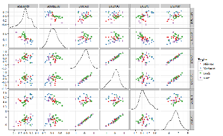
Figure 5. Trellis plot, correlations among variables.
A matrix of partial correlations was produced from the Rcmdr correlation call. Thus, to pick just one partial correlation, the association between DEMOCRATS and RELIGION (reported as “very important”) is negative (r = -0.45) and from the second matrix we retrieve the approximate P-value, unadjusted for the multiple comparisons problem, of p = 0.0024. We quickly move past this matrix to the adjusted P-values and confirm that this particular correlation is statistically significant even after correcting for multiple comparisons. Thus, there is a moderately strong negative correlation between those who reported that religion was very important to them and the difference between registered Democrats and Republicans in the 48 states. Because it is a partial correlation, we can conclude that this correlation is independent of all of the other included variables.
And what about our original question: Do Democrats prefer cats over dogs? The partial correlation after adjusting for all of the other correlated variables is small (r = 0.05) and not statistically different from zero (P-value greater than 5%).
Are there any interesting associations involving pet ownership in this data set? See if you can find it (hint: the correlation you are looking for is also in red).
Partial correlations:
         ASDEMS  ASRELIG LGCAT   LGDOG   LGIPC   LGPOP
ASDEMS   0.0000 -0.4460  0.0487  0.0605  0.1231 -0.0044
ASRELIG -0.4460  0.0000 -0.2291 -0.0132 -0.4685  0.2659
LGCAT    0.0487 -0.2291  0.0000  0.2225 -0.1451  0.6348
LGDOG    0.0605 -0.0132  0.2225  0.0000 -0.6299  0.5953
LGIPC    0.1231 -0.4685 -0.1451 -0.6299  0.0000  0.6270
LGPOP   -0.0044  0.2659  0.6348  0.5953  0.6270  0.0000
Raw P-values, Pairwise two-sided p-values:
         ASDEMS ASRELIG  LGCAT   LGDOG   LGIPC   LGPOP
ASDEMS           0.0024  0.7534  0.6965  0.4259  0.9772
ASRELIG  0.0024          0.1347  0.9325  0.0013  0.0810
LGCAT    0.7534  0.1347          0.1465  0.3473  <.0001
LGDOG    0.6965  0.9325  0.1465          <.0001  <.0001
LGIPC    0.4259  0.0013  0.3473  <.0001          <.0001
LGPOP    0.9772  0.0810  <.0001  <.0001  <.0001
Adjusted P-values, Holm’s method (Benjamini and Hochberg 1995)
         ASDEMS ASRELIG  LGCAT   LGDOG   LGIPC   LGPOP
ASDEMS           0.0241  1.0000  1.0000  1.0000  1.0000
ASRELIG  0.0241          1.0000  1.0000  0.0147  0.7293
LGCAT    1.0000  1.0000          1.0000  1.0000  <.0001
LGDOG    1.0000  1.0000  1.0000          <.0001  0.0002
LGIPC    1.0000  0.0147  1.0000  <.0001          <.0001
LGPOP    1.0000  0.7293  <.0001  0.0002  <.0001
A graph (Fig 6) to summarize the partial correlations: green lines indicate positive correlation, red lines show negative correlations; Strength of association indicated by the line thickness, with thicker lines corresponding to greater correlation.
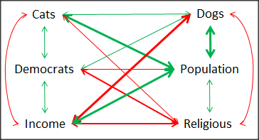
Figure 6. Causal paths among variables.
As you can see, partial correlation analysis is good for a few variables, but as the numbers increase it is difficult to make heads or tails out of the analysis. Better methods for working with these highly correlated data in what we call multivariate data analysis, for example Structural Equation Modeling or Path Analysis.
Questions
- Write up three learning outcomes for this page. Hint: Point your favorite generative AI to this page and ask for help.
- Spurious correlations can be challenging to recognize, and, sometimes, they become part of a challenge to medicine to explain away. A classic spurious correlation is the correlation between rates of MMR vaccination and autism prevalence. Here’s a table of numbers for you
| Year | Herb Supplement Revenue, millions $ | Fertility rate per 1000 births, women age 35 and older+ | MMR per 100K children age 0 -5 | UFC revenue, millions $ | Autism Prevalence per 1000 |
|---|---|---|---|---|---|
| 2000 | 4225 | 47.7 | 179 | 6.7 | |
| 2001 | 4361 | 48.6 | 183 | 4.5 | |
| 2002 | 4275 | 49.9 | 190 | 8.7 | 6.6 |
| 2003 | 4146 | 52.6 | 196 | 7.5 | |
| 2004 | 4288 | 54.5 | 199 | 14.3 | 8 |
| 2005 | 4378 | 55.5 | 197 | 48.3 | |
| 2006 | 4558 | 56.9 | 198 | 180 | 9 |
| 2007 | 4756 | 57.6 | 204 | 226 | |
| 2008 | 4800 | 56.7 | 202 | 275 | 11.3 |
| 2009 | 5037 | 56.1 | 201 | 336 | |
| 2010 | 5049 | 56.1 | 209 | 441 | 14.4 |
| 2011 | 5302 | 57.5 | 212 | 437 | |
| 2012 | 5593 | 58.7 | 216 | 446 | 14.5 |
| 2013 | 6033 | 59.7 | 220 | 516 | |
| 2014 | 6441 | 61.6 | 224 | 450 | 16.8 |
| 2015 | 6922 | 62.8 | 222 | 609 | |
| 2016 | 7452 | 64.1 | 219 | 666 | 18.5 |
| 2017 | 8085 | 63.9 | 213 | 735 | |
| 2018 | 65.3 | 220 | 800 | 25 |
- Make scatterplots of autism prevalence vs
- Herb supplement revenue
- Fertility rate
- MMR vaccination
- UFC revenue
- Calculate and test correlations between autism prevalence vs
- Herb supplement revenue
- Fertility rate
- MMR vaccination
- UFC revenue
- Interpret the correlations — is there any clear case for autism vs MMR?
- What additional information is missing from Table 2? Add that missing variable and calculate partial correlations for autism prevalence vs
- Herb supplement revenue
- Fertility rate
- MMR vaccination
- UFC revenue
- Do a little research: What are some reasons for increase in autism prevalence? What is the consensus view about MMR vaccine and risk of autism?
Quiz Chapter 16.2
Causation and Partial correlation
Data sets
Data used in this page, 100 meter running times since 1900.
| Year | Men | Women |
|---|---|---|
| 1912 | 10.6 | |
| 1913 | ||
| 1914 | ||
| 1915 | ||
| 1916 | ||
| 1917 | ||
| 1918 | ||
| 1919 | ||
| 1920 | ||
| 1921 | 10.4 | |
| 1922 | 13.6 | |
| 1923 | 12.7 | |
| 1924 | ||
| 1925 | 12.4 | |
| 1926 | 12.2 | |
| 1927 | 12.1 | |
| 1928 | 12 | |
| 1929 | ||
| 1930 | 10.3 | |
| 1931 | 12 | |
| 1932 | 11.9 | |
| 1933 | 11.8 | |
| 1934 | 11.9 | |
| 1935 | 11.9 | |
| 1936 | 10.2 | 11.5 |
| 1937 | 11.6 | |
| 1938 | ||
| 1939 | 11.5 | |
| 1940 | ||
| 1941 | ||
| 1942 | ||
| 1943 | 11.5 | |
| 1944 | ||
| 1945 | ||
| 1946 | ||
| 1947 | ||
| 1948 | 11.5 | |
| 1949 | ||
| 1950 | ||
| 1951 | ||
| 1952 | 11.4 | |
| 1953 | ||
| 1954 | ||
| 1955 | 11.3 | |
| 1956 | 10.1 | |
| 1957 | ||
| 1958 | 11.3 | |
| 1959 | ||
| 1960 | 10 | 11.3 |
| 1961 | 11.2 | |
| 1962 | ||
| 1963 | ||
| 1964 | 10.06 | 11.2 |
| 1965 | 11.1 | |
| 1966 | ||
| 1967 | 11.1 | |
| 1968 | 9.9 | 11 |
| 1969 | ||
| 1970 | 11 | |
| 1972 | 10.07 | 11 |
| 1973 | 10.15 | 10.9 |
| 1976 | 10.06 | 11.01 |
| 1977 | 9.98 | 10.88 |
| 1978 | 10.07 | 10.94 |
| 1979 | 10.01 | 10.97 |
| 1980 | 10.02 | 10.93 |
| 1981 | 10 | 10.9 |
| 1982 | 10 | 10.88 |
| 1983 | 9.93 | 10.79 |
| 1984 | 9.96 | 10.76 |
| 1987 | 9.83 | 10.86 |
| 1988 | 9.92 | 10.49 |
| 1989 | 9.94 | 10.78 |
| 1990 | 9.96 | 10.82 |
| 1991 | 9.86 | 10.79 |
| 1992 | 9.93 | 10.82 |
| 1993 | 9.87 | 10.82 |
| 1994 | 9.85 | 10.77 |
| 1995 | 9.91 | 10.84 |
| 1996 | 9.84 | 10.82 |
| 1997 | 9.86 | 10.76 |
| 1998 | 9.86 | 10.65 |
| 1999 | 9.79 | 10.7 |
| 2000 | 9.86 | 10.78 |
| 2001 | 9.88 | 10.82 |
| 2002 | 9.78 | 10.91 |
| 2003 | 9.93 | 10.86 |
| 2004 | 9.85 | 10.77 |
| 2005 | 9.77 | 10.84 |
| 2006 | 9.77 | 10.82 |
| 2007 | 9.74 | 10.89 |
| 2008 | 9.69 | 10.78 |
| 2009 | 9.58 | 10.64 |
| 2010 | 9.78 | 10.78 |
| 2011 | 9.76 | 10.7 |
| 2012 | 9.63 | 10.7 |
| 2013 | 9.77 | 10.71 |
| 2014 | 9.77 | 10.8 |
| 2015 | 9.74 | 10.74 |
| 2016 | 9.8 | 10.7 |
| 2017 | 9.82 | 10.71 |
| 2018 | 9.79 | 10.85 |
| 2019 | 9.76 | 10.71 |
| 2020 | 9.86 | 10.85 |
| 2021 | 9.77 | 10.54 |
| 2022 | 9.76 | 10.62 |
| 2023 | 9.83 | 10.65 |
| 2024 | 9.77 | 10.72 |
Data used in this page, birth weight by lead exposure
| CityTown | Core | Population | NTested | HiLead | Births | LowBirthWeight | InfantDeaths |
|---|---|---|---|---|---|---|---|
| Barrington | n | 16819 | 237 | 13 | 785 | 54 | 1 |
| Bristol | n | 22649 | 308 | 24 | 1180 | 77 | 5 |
| Burrillville | n | 15796 | 177 | 29 | 824 | 44 | 8 |
| Central Falls | y | 18928 | 416 | 109 | 1641 | 141 | 11 |
| Charlestown | n | 7859 | 93 | 7 | 408 | 22 | 1 |
| Coventry | n | 33668 | 387 | 20 | 1946 | 111 | 7 |
| Cranston | n | 79269 | 891 | 82 | 4203 | 298 | 20 |
| Cumberland | n | 31840 | 381 | 16 | 1669 | 98 | 8 |
| East Greenwich | n | 12948 | 158 | 3 | 598 | 41 | 3 |
| East Providence | n | 48688 | 583 | 51 | 2688 | 183 | 11 |
| Exeter | n | 6045 | 73 | 2 | 362 | 6 | 1 |
| Foster | n | 4274 | 55 | 1 | 208 | 9 | 0 |
| Glocester | n | 9948 | 80 | 3 | 508 | 32 | 5 |
| Hopkintown | n | 7836 | 82 | 5 | 484 | 34 | 3 |
| Jamestown | n | 5622 | 51 | 14 | 215 | 13 | 0 |
| Johnston | n | 28195 | 333 | 15 | 1582 | 102 | 6 |
| Lincoln | n | 20898 | 238 | 20 | 962 | 52 | 4 |
| Little Compton | n | 3593 | 48 | 3 | 134 | 7 | 0 |
| Middletown | n | 17334 | 204 | 12 | 1147 | 52 | 7 |
| Narragansett | n | 16361 | 173 | 10 | 728 | 42 | 3 |
| Newport | y | 26475 | 356 | 49 | 1713 | 113 | 7 |
| New Shoreham | n | 1010 | 11 | 0 | 69 | 4 | 1 |
| North Kingstown | n | 26326 | 378 | 20 | 1486 | 76 | 7 |
| North Providence | n | 32411 | 311 | 18 | 1679 | 145 | 13 |
| North Smithfield | n | 10618 | 106 | 5 | 472 | 37 | 3 |
| Pawtucket | y | 72958 | 1125 | 165 | 5086 | 398 | 36 |
| Portsmouth | n | 17149 | 206 | 9 | 940 | 41 | 6 |
| Providence | y | 173618 | 3082 | 770 | 13439 | 1160 | 128 |
| Richmond | n | 7222 | 102 | 6 | 480 | 19 | 2 |
| Scituate | n | 10324 | 133 | 6 | 508 | 39 | 2 |
| Smithfield | n | 20613 | 211 | 5 | 865 | 40 | 4 |
| South Kingstown | n | 27921 | 379 | 35 | 1330 | 72 | 10 |
| Tiverton | n | 15260 | 174 | 14 | 516 | 29 | 3 |
| Warren | n | 11360 | 134 | 17 | 604 | 42 | 1 |
| Warwick | n | 85808 | 973 | 60 | 4671 | 286 | 26 |
| Westerly | n | 22966 | 140 | 11 | 1431 | 85 | 7 |
| West Greenwich | n | 5085 | 68 | 1 | 316 | 15 | 0 |
| West Warwick | n | 29581 | 426 | 34 | 2058 | 162 | 17 |
| Woonsoket | y | 43224 | 794 | 119 | 2872 | 213 | 22 |
Data in this page, Do Democrats prefer cats?
Chapter 16 contents
- Introduction
- Product moment correlation
- Causation and Partial correlation
- Data aggregation and correlation
- Spearman and other correlations
- Instrument reliability and validity
- Similarity and Distance
- References and suggested readings
5 – Experimental design
Beyond numbers.
During this course, you will learn about statistics, yes, but my hope and goal for your experience in this class is much more than that: statistical reasoning. To have statistical reasoning skills, you need to be comfortable with the context of how data are acquired, ie, data acquisition. It’s not just about knowing how an instrument performs, eg, under or over the limits of quantification characteristics of the instrument lead to censored missing values, missing not at random (MNAR). In a broad stoke view, data are obtained from two kinds of studies: observational studies and experimental (manipulative) studies. what a correctly designed experiment can tell you about the world, and how a poorly designed experiment works against you. At the end of the semester, you should be familiar with the issues of Randomization, Control, Independence, and Replication.
The basics explained.
Experimental design is a discipline within statistics concerned with the analysis and design of experiments. Design is intended to help research create experiments such that cause and effect can be established from tests of the hypothesis. We introduced elements of experimental design in Chapter 2.4. I recommend a quick re-read: We talk about the different types of bias that can affect research. We also point out parts of the problem you’ll need to think about when planning a project, so you can avoid or reduce bias from the start.
Note 1: Just the highlights from Chapter 2.4: use randomization, blinding, and control measures in the study design. Different strategies may be needed depending on the type of bias.
Here, we expand our discussion of experimental design. We begin with review of definitions and an outline of an important concept in statistics. First, we need to be clear about why we measure or conduct experiments. We do so to collect data (datum is the singular) about a characteristic or trait from a population. Data are observations: they include observations and measurements from instruments. At their best, data are the “facts” of science.
Measurement, Observation, Variables, Values.
Measurement is how we as scientists acquire our data (Chapter 3.4). The process of measuring involves the assignment of numbers, codes, or labels to observations according to rules established prior to any data collection (Stevens 1946, Houle et al 2011). Observations refer to the units of measurement, whereas variables are the characteristics or traits that are measured. A value refers to the particular number, score, or label assigned to a particular sample for a variable. Variables are generic, the thing being measured, values are specific to the subject or sample being measured for the variable. Each discipline in biology has its own set of variables and samples may or may not have different values for each variable measured. Variables are summarized as a statistic (eg, the sample mean), which is a number taken to estimate a parameter, which pertains to the population. Variables and parameters in statistics were discussed in Chapter 3.4. Because numbers or scores or labels can be assigned according to different rules, this means that variables may be measured on different kinds of scales or data types. The different kinds of data types were presented in Chapter 3.1.
Missing values.
A missing value refers to lack of a value for an observation or variable (Chapter 3.5). Censored values, a type of missing value, include observations for which limited or partial information is available, eg, range, while a missing value lacks any information about the true value.
Missing values can affect analysis and many R algorithms are sensitive or may fail to run in the presence of missing values. Missing data may be of three kinds, and one of them, missing not at random (MNAR), can substantially influence the analysis. MNAR implies some observations are missing because of a systematic bias. Instrument limits of quantification are an example of systematic bias — for example, spectrophotometric absorbance readings of zero for a colorimetric assay (eg, Bradford protein assay) may not represent complete absence of the target, but rather, the lower detection limits of the instrument or the assay method (0.1 mg protein/mL in this case).
The other kinds of missing values are missing completely at random (MCAR) and missing at random (MAR). MCAR implies there is no association between any element of the experiment and the absence of a value. Analysis on MCAR data sets may support unbiased conclusions. MAR includes the random errors that occur during data acquisition: data may be lost because of operator error or power outage (shudder). Unlike MNAR, analysis of MAR, like MCAR data sets may still result in unbiased conclusions.
Note 2: The word “may” is doing some heavy lifting here; obviously, the size of the data set influences whether this claim holds.
One consequence of missing values — a decision how best to handle the lost information. The options are either pairwise deletion or listwise deletion. Listwise means the entire row, all variables, are lost for any record with one or more missing values. You recorded root length, stem length, numbers of secondary roots, time to germinate, but the SPAD meter failed and there is no chlorophyl reading for seedling #212? Sorry, the entire row is deleted. Optionally, the missing data is deleted pairwise — only chlorophyl reading for #212 is lost, all other variables remain.
Users of R will quickly learn some algorithms immediately fail to run if not instructed how to process missing values. In some cases, missing values can be replaced by imputed values.
Note 3: This being an introduction to applied biostatistics, we won’t dwell on the pros and cons of imputation. Instead, I point interested readers to two heavily cited articles: Schafer 1999; Schafer and Graham 2002.
Cause & Effect.
Observations or measurements gathered under controlled conditions (experiments) are essential if we are to answer questions about populations, to separate cause and effect, where one or more events is directly the result of another factor, as opposed to anecdote, a story about an event which, by itself, cannot be used to cause from association (eg, spurious correlations, see Ch 16.2). Recall that anecdotal evidence typically comes from personal experience, where observations may be obtained by non-systematic methods. Well designed experiments, in the classical sense, permit discrimination among competing hypotheses in large part because observations are collected according to strict rules. Well developed hypotheses tested by well-designed experiments permit ruling out alternative explanations (sensu Pratt [1964] strong inference). Observational studies, or epidemiology studies if we are talking about investigations of risk assessment, also may contribute to discussions of cause and effect (see history of smoking by Doll 1998).
Medicine is replete with stories about how a patient showed a particular set of symptoms, and how a physician applied a set of diagnostic protocols. An outcome was achieved, and the physician reports the outcome and circumstances related to the patient to her colleagues. This is an example of a case study, and the focus of investigation is the individual, the patient. The doctor’s report will sound like, “I tried the standard treatment given the diagnosis, and the patient’s symptoms diminished, but later returned. I tried a higher dose, but the patient’s symptoms persisted unabated.” No inferences are made to a wider set of individuals and the report is anecdotal. If observations are made on several patients, this may be a case series.
In ecology, a field biologist may notice a six-legged adult frog (Scott 1999, Alvarez et al 2021) — since frogs typically have four legs, the six-legged frog attracts the biologist’s eye and he jots down the circumstances in which the frog were found: relative humidity, air temperature, ground temperature, where the frogs was found (on lower leaf of a philodendron plant). A water source near where the frog was found is tested for pH with a meter the biologist carries, and a water sample is taken for later testing of herbicides. The frog is collected so that it can be checked for skin parasites. Upon further inspection, the frog did indeed have parasites known to cause deformities in other frog species. However, note that this example too, is a case study. Although the biologist makes additional observations, any conclusions about why the frog has six legs is anecdotal.
From these case studies, no conclusions can be drawn. We cannot say why the patient failed to respond to treatment, nor can we say why the frog has six legs. Why? Because these are singular events, and a variety of explanations can be given as to their causes — importantly, no controls are available, so there’s no way to distinguish among possibilities.
From such anecdotes, however, experiments can be designed. The physician may decide to recruit additional patients with the diagnosed illness and apply the standard treatment to see if her anecdote is a single, unique event, or more indicative of a problem with the treatment. The biologist may collect other frogs from the area near where he found the six-legged frog and check to see if they, too, have the parasites. If additional patients fail to respond to the treatment, then the singular even is more likely to be a phenomenon. If the normal frogs also have similar levels of the parasite then it is unlikely that these parasites caused the malformed frog. With this simple step (recruiting similar patients, finding additional frogs), we can begin to make inferences about cause and effect and in some cases, to generalize our findings.
This is the objective of most statistical procedures, the concept of sampling from a reference population and making distinctions between groups within the sample. The difference between observational and experimental studies then is how the subjects are selected with respect to the groups. In an experiment, the researcher controls and decides which subject receives the treatment, therefore, allocation to groups is manipulated by the researcher. In contrast, subjects included in an observational study have already been “assigned” to a group, but not by us. Assignment to groups, smokers or non smokers, Type II diabetes or no diabetes (etc.), is done by nature.
Now, I do not wish to imply that research that cannot be generalized back to a reference population are worthless. Far from it. In fact, there is a strong argument for specificity. For example, much basic biological research depends on work or model organisms, which in turn may be further partitioned into specific genetic lines (cf. discussion in Rothman et al 2013). And my goodness, what we have learned about the devastation to oceanic islands like Guam when the brown tree snake was introduced (Fritts and Rodda 1998). Strictly speaking, what has happened to Guam is a case history. But no one would argue that what has happened to Guam cannot happen to Hawaii and other oceanic islands (eg, United States Federal law 384-108 “Brown Tree Snake Control and Eradication Act of 2004”). In other words, even from case histories, generalizations can sometimes be made.
There can also be real reasons to ignore the issue of generality. One benefit of specificity is experimental control. Transgenic lines may differ by single gene knockout or by gene duplication, and clearly the aim of such studies is to evaluate the function (hence purpose) of the gene product (or its absence) on some phenotype. In this sense it may not seem important that an transgenic mouse is not representative of a wild outbred mouse population. However, this argument is fundamentally one of expedience — such studies do result in specific results, results that cannot be generalized beyond the strains involved. It ignores the issue of genetic background — all of the genes that affect a trait in addition to the candidate gene under study (Sigmund 2000; Lariviere et al 2001). Transgenic mice of different inbred strains or their hybrids may have very different alleles at other genes that may influence a phenotype, hence, the results of the gene knockdown or other engineering result in different outcomes. Results of genetic manipulations on inbred strains, no matter how sophisticated, the conclusions are strain- or hybrid cross-specific. Thus, although technically and financially difficult, conclusions are better, more generalizable, when conducted with many different inbred lines and verified in outbred mouse populations precisely because genetic background often influences function of single genes (Sigmund 2000; Lariviere et al 2001).
“Causal criteria:” Logic of causation in medicine.
This section is in progress. Just a list of key points and references
Throughout this text, emphasis on the power of experimentation is emphasized. Well designed experiments …
Henle-Koch’s postulates (1877, 1882), working on tuberculosis reported a set of causal criteria to establish link between a microorganism and a disease, are the following:
- The microorganism must be found in abundance in all organisms suffering from the disease, but should not be found in healthy organisms.
- The microorganism must be isolated from a diseased organism and grown in pure culture.
- The cultured microorganism should cause disease when introduced into a healthy organism.
- The microorganism must be reisolated from the inoculated, diseased experimental host and identified as being identical to the original specific causative agent.
Robert Koch wrote these more than 100 years ago, so, clearly, understanding of infectious disease has improved. Evan’s postulates, quoted from A Dictionary of Epidemiology, 5th edition (pp. 86-87).
- Prevalence of the disease should be significantly higher in those exposed to the hypothesized cause than in controls not so exposed.
- Exposure to the hypothesized cause should be more frequent among those with the disease than in controls without the disease—when all other risk factors are held constant.
- Incidence of the disease should be significantly higher in those exposed to the hypothesized cause than in those not so exposed, as shown by prospective studies.
- The disease should follow exposure to the hypothesized causative agent with a normal or log-normal distribution of incubation periods.
- A spectrum of host responses should follow exposure to the hypothesized agent along a logical biological gradient from mild to severe.
- A measurable host response following exposure to the hypothesized cause should have a high probability of appearing in those lacking this before exposure (eg, antibody, cancer cells) or should increase in magnitude if present before exposure. This response pattern should occur infrequently in persons not so exposed.
- Experimental reproduction of the disease should occur more frequently in animals or humans appropriately exposed to the hypothesized cause than in those not so exposed; this exposure may be deliberate in volunteers, experimentally induced in the laboratory, or may represent a regulation of natural exposure.
- Elimination or modification of the hypothesized cause should decrease the incidence of the disease (eg, attenuation of a virus, removal of tar from cigarettes).
- Prevention or modification of the host’s response on exposure to the hypothesized cause should decrease or eliminate the disease (eg, immunization, drugs to lower cholesterol, specific lymphocyte transfer factor in cancer).
- All of the relationships and findings should make biological and epidemiological sense.
Fredericks, D. N., & Relman, D. A. (1996). Sequence-based identification of microbial pathogens: a reconsideration of Koch’s postulates. Clinical microbiology reviews, 9(1), 18-33.
Correlation (association) does not imply causation, a well-worn truism in any application of critical thinking skills. Conversely, causation does imply association (correlation); If a change in one variable directly changes another variable, there will be a statistical association between the two variables. Thus, a correlation between two variables is necessary, but not sufficient evidence for cause and effect between two variables.
Note 4: Association is the more general term for a possible relationship between two or more variables. A correlation in statistics generally refers to a linear association (Chapter 16); the aforementioned truism should be restated as association (or statistical relationship) does not imply causation.
However, sometimes association does point to a cause. A familiar example is association between tobacco cigarette smoking causes lung cancer. Surgeon General Luthar Terry’s 1964 report (link to document in National Library of Medicine), presented a strong case linking smoking to elevated risk of lung cancer and coronary artery disease.
Bradford Hill’s guidelines to evaluate causal effects based on epidemiology (Hill 1965, see also Sussar 1999, Fedak et al 2015). Set of necessary and sufficient conditions, inductive reasoning.
- Strength of association
- Consistency of observed association
- Specificity of association
- Temporal relationship of the association
- Biological gradient, eg, a dose-response curve
- Biological plausibility
- Coherence, the cause and effect inference should not conflict with what is known about the etiology of a disease.
Follows and extends David Hume’s (1739) causation criteria: association (Hill #1), cause precedes effect (Hill #4), direction of connection.
Validity.
An obvious objective of research is to reach valid conclusions about fundamental questions. A helpful distinction between the specific and the generalizable experiment is to recognize there are two forms of validity in research: internal validity and external validity (Elwood 2013). Internal validity is the quality of a designed study that determines whether cause and effect can be determined. Random assignment of subjects to treatment groups enhances the internal validity of the study. External validity relates to how general the assessment of cause and effect can be to other populations. Thus, random sampling from a reference population has to do with whether or not the study has external validity.
Additional definitions.
We proceed now with definitions. We use the term population in a special and restrictive way in statistics. Our definition includes the one you are already familiar with, but it also means more than that.
Populations are the entire group of individuals that you want to investigate. In statistics, the entire groups is actually the entire class with the observation — so if we are referring to the average body weight of house mice, we’re actually referring to the body weight as the population — it’s a subtle distinction, not essential for our introduction to biostatistics. When we conduct experiments and apply statistical tests on collected data, we generally intend to make inferences (draw conclusions) from our results back to the population.
Population has a strict application in statistics, but the definition also includes our general understanding of the word population. For example, Examples of a population in the general sense one may refer to include: .… the entire human population existing today .… the entire collection of U.S. citizens. .… all the individuals in an entire species. .… all individuals in a population of a species (eg, house mice in a dairy barn in Hawai’i) .… all of us in this classroom (if we are ONLY interested in US) If you could measure the entire population then there would be no need to do (or learn) statistics! Populations usually are in the thousands, millions, or billions of individuals. Here, population is used in the everyday sense that we think of — a collection of individuals that share a characteristic.
A more formal definition of “population” in statistics reads as follows: A statistical population is the complete set of possible measurements on a trait or characteristic corresponding to the entire collection of sampling units for which conclusions are intended.
To conclude, in this class, when we talk about population, we will generally be using it in the everyday sense of the word. However, keep in mind that the definition is more restrictive than that and the key is to identify what sampling units are measured.
Conclusions.
This is only the beginning, the basics of experimental design. Beginning with RA Fisher‘s 1935 book, The Design of Experiments (nine editions, some freely accessible via internet search), which is still very much worth reading, entire books are written on the subject, as you can well imagine.
Note 5: Fisher’s The Design of Experiments concerned experimental design, randomization, blocking, and replication, particularly from perspective of agriculture research. Most readers of this eBook likely know that RA Fisher’s broader career absolutely included eugenics and hereditarian views about human populations and race. Those views are not in The Design of Experiments, which is largely about methods and statistical framework for inference.
We will also return to the subject of Experimental Design throughout the book. We will return to random sampling in Chapter 5.5. Next we discuss distinctions between experiments and observational studies with respect to sampling of populations.
A bit of a disclaimer here before proceeding; while I cite several papers for examples in experimental design in Chapter 5, reader’s should not read into this that I am either criticizing or endorsing the published experiments. Experimental design will always have elements of compromise — the trick of course is knowing which choices influence validity (Thompson and Panacek 2006).
Questions.
- Define in your own words the following terms
- reference population
- subjects
- specific versus general conclusions
- random sampling
- convenience sampling
- haphazard sampling
- research validity
- Revisit our cell experiment, “What is the sampling unit in the following cell experiment?” How would you change this experiment so that there will be biological and not just technical replication?
- Describe the type of sampling for each research scenario described?
- All African snails on a staircase at Chaminade University are collected on a Thursday evening.
- All African snails on a staircase at Chaminade University are collected every Thursday evening for six months.
- All African snails on all staircases at Chaminade University are collected.
- African snails are studied in the lab, then returned to the areas from which they were collected. Days later, the researcher collects snails from the same area.
- African snails are studied in the lab, then returned to the areas from which they were collected. Days later, the researcher collects snails from a different area.
- The Chaminade University campus is divided into grids. Grids that include stairwells are marked. Before collecting snails, the researcher randomly selects from the list of grids and searches for snails only in those grids selected from the list.
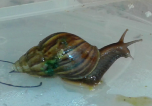
Figure 1. Giant African Snail (Lissachatina fulica, formerly Achatina fulica). Image by M. Dohm.
- This next scenario may be evaluated by you for potential sources of bias. Review the list of bias listed above. A researcher wants to do a population count of feral cats on campus. Feral cats are active at night, so he decides to set up a feeding station near a light post. The researcher sits all night in a parked car yards away and watches the feeding station for visits by cats. The researcher repeats these observations over the course of a week, moving the feeding station to different campus locations each night, and reports the total number of cats seen during the week as an estimate of the population size. Be able to discuss this study in terms of potential and actual bias.
Quiz
Including the quiz on this page, a total of 65 questions among the several subchapters, a mix of true or false and multiple choice question format.
Quiz Chapter 5
Experimental design