17 – Linear Regression
Introduction
Regression is a toolkit for developing models of cause and effect between one ratio scale data type dependent response variables, and one (simple linear regression) or more or more (multiple linear regression) ratio scale data type independent predictor variables. By convention the dependent variable(s) is denoted by Y, the independent variable(s) represented by X1, X2,  Xn for n independent variables. Like ANOVA, linear regression is simply a special case of the general linear model, first introduced in Chapter 12.7.
Components of a statistical model
Regression statistical methods return model estimates of the intercept and slope coefficients, plus statistics of regression fit (eg, R2, aka “R-squared,” the coefficient of determination).
Chapter 17.1 – 17.9 cover the simple linear model

Chapter 18.1 – 18.5 cover the multiple regression linear model

where α or β0 represent the Y-intercept and β or β1, β2, … βn represent the regression slopes.
Regression and correlation test linear hypotheses
We state that the relationship between two variables is linear (the alternative hypothesis) or it is not (the null hypothesis). The difference? Correlation is a test of linear association (are variables correlated, we ask?), imply possible causation, but are not sufficient evidence for causation: we do not imply that one variable causes another to vary, even if the correlation between the two variables is large and positive, for example. Correlations are used in statistics on data sets not collected from explicit experimental designs incorporated to test specific hypotheses of cause and effect.
Linear regression, however, is to cause and effect as correlation is to association. With regression and ANOVA, we are indeed making a case for a particular understanding of the cause of variation in a response variable: modeling cause and effect is the goal. Regression, ANOVA, and other general linear models are designed to permit the statistician to control for the effects of confounding variables provided the causal variables themselves are uncorrelated.
When to use correlation and when to apply linear regression to data set? For two ratio scale variables, one can always apply either approach. Correlation is always appropriate if both variables are measured in the course of the study whereas a regression modeling approach would be implied where one variable was the result of manipulation by the researcher.
Assumptions of linear regression
The key assumption in linear regression is that a straight line indeed is the best fit of the relationship between dependent and independent variables. The additional assumptions of parametric tests (Chapter 13) also hold. In Chapter 18 we conclude with an extension of regression from one to many predictor variables and the special and important topic of correlated predictor variables or multicollinearity.
Build a statistical model, make predictions
In our exploration of linear regression we begin with simple linear regression, also called ordinary least squares regression, starting with one predictor variable. Practical aspects of model diagnostics are presented. Regression may be used to describe or to provide a predictive statistical framework. In Chapter 18 we conclude with an extension of regression from one to many predictor variables. We conclude with a discussion of model selection. Throughout, use of Rcmdr and R have multiple ways to analyze linear regression models are presented; we will continue to emphasize the general linear model approach, but note that use of linear model in Rcmdr provides a number of default features that are conveniently available.
Questions
1. Write up three learning outcomes for this page. Hint: Point your favorite generative AI to this page and ask for help.
Suggested homework
Homework 11: Simple linear regression.
Quiz
In addition to the quiz on this page, a total of 81 questions among the several subchapters, a mix of true or false and multiple choice question format.
Quiz Chapter 17
Linear Regression
References
Linear regression is a huge topic; references I include are among my favorite on the subject, but are only a small and incomplete sampling. For simplicity, I merged references for Chapter 17 and Chapter 18 into one page at References and suggested readings (Ch17 & 18)
Chapter 17 contains
- Introduction
- Simple Linear Regression
- Relationship between the slope and the correlation
- Estimation of linear regression coefficients
- OLS, RMA, and smoothing functions
- Testing regression coefficients
- ANCOVA – analysis of covariance
- Regression model fit
- Assumptions and model diagnostics for Simple Linear Regression
- References and suggested readings (Ch17 & 18)
14.4 – Randomized block design
Introduction
Randomized Block Designs and Two-Factor ANOVA
In previous lectures, we have introduced you to the standard factorial ANOVA, which may be characterized as being crossed, balanced, and replicated. We expect additional factors (covariates) may contribute to differences among our experimental units, but rather than testing them — which would increase need for additional experimental units because of increased number of groups to test — we randomize our subjects. Randomization is intended to disrupt trends of confounding variables (aka covariates). If the resulting experiment has missing values (see Chapter 5), then we can say that the design is partially replicated; if only one observation is made per group, then the design is not replicated — and perhaps, not very useful!!
A special type of Two-factor ANOVA which includes a “blocking” factor and a treatment factor.
Randomization is one way to control for “uninteresting” confounding factors. Clearly, there will be scenarios in which randomization is impossible. For example, it is impossible to randomly assign subjects to The blocking factor is similar to the 10.3 – Paired t-test. In the paired t-test we had two individuals or groups that we paired (eg, twins). One specific design is called the Randomized Block Design and we can have more than 2 members in the group. We arrange the experimental units into similar groups, ie, the blocking factor. Examples of blocking factors may include day (experiments are run over different days), location (experiments may be run at different locations in the laboratory), nucleic acid kits (different vendors), operator (different assistants may work on the experiments), etcetera.
In general we may not be directly interested in the blocking factor. This blocking factor is used to control some factor(s) that we suspect might affect the response variable. Importantly, this has the effect of reducing the sums of squares by an amount equal to the sums of squares for the block. If variability removed by the blocking is significant, Mean Square Error (MSE) will be smaller, meaning that the F for treatment will be bigger — meaning we have a more powerful ANOVA than if we had ignored the blocking.
Statistical Testing in Randomized Block Designs
“Blocks” is a Random Factor because we are “sampling” a few blocks out of a larger possible number of blocks. Treatment is a Fixed Factor, usually.
The statistical model is

The Sources of Variation are simpler than the more typical Two-Factor ANOVA because we do not calculate all the sources of variation – the interaction is not tested! (Table 1).
Table 1. Sources of variation for a two-way ANOVA, randomized block design
|
Sources of Variation & Sum of Squares
|
DF
|
Mean Squares
|
 |
 |
 |
 |
 |
 |
 |
 |
 |
 |
 |
 |
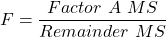
Critical Value F0.05(2), (a – 1), (Total DF – a – b)
In the exercise example above: Factor A = exercise or management plan.
Notice that we do not look at the interaction MS or the Blocking Factor (typically).
Learn by doing
Rather than me telling you, try on your own. We’ll begin with a worked example, then proceed to introduce you to three problems. Click here (Ch 14.8)for general discussion of Rcmdr and linear models for models other than the standard 2-way ANOVA (Chapter 14.8).
Worked example
Wheel running by mice is a standard measure of activity behavior. Even wild mice will use wheels (Meijer and Roberts 2014). For example, we conduct a study of family parity to see if offspring from the first, second, or third sets of births from wheel-running behavior in mice (total revs per 24 hr period). Each set of offspring from a female could be treated as a block. Data are for 3 female offspring from each pairing. This type of data set would look like this:
Table 2. Wheel running behavior by three offspring from each of three birth cohorts among four maternal sets (moms).
|
Revolutions of wheel per 24-hr period
|
||||
|
Block
|
Dam 1
|
Dam 2
|
Dam 3
|
Dam 4
|
|
b1
|
1100
|
1566
|
945
|
450
|
|
b1
|
1245
|
1478
|
877
|
501
|
|
b1
|
1115
|
1502
|
892
|
394
|
|
b2
|
999
|
451
|
644
|
605
|
|
b2
|
899
|
405
|
650
|
612
|
|
b2
|
745
|
344
|
605
|
700
|
|
b3
|
1245
|
702
|
1712
|
790
|
|
b3
|
1300
|
612
|
1745
|
850
|
|
b3
|
1750
|
508
|
1680
|
910
|
Thus, there were nine offspring for each female mouse (Dam1 – Dam4), three offspring per each of three litters of pups. The litters are the blocks. We need to get the data stacked to run in R. I’ve provided the full dataset for readers, scroll to end of this page or click here.
Question 1. Describe the problem and identify the treatment and blocking factors.
Answer. Each female has three litters. We’re primarily interested in genetics (and maternal environment) of wheel running behavior, which is associated with the moms (Treatment factor). The questions is whether there is an effect of birth parity on wheel running behavior. Offspring of a first-time mother may experience different environment than offspring of experienced mother. In this case, parity effects is an interesting question, nevertheless, blocking is the appropriate way to handle this type of problem.
Question 2. What is the statistical model?
Answer. Response variable, Y, is wheel running. Let α the effect of Dam and β the birth cohorts (ie, the blocking effect).
Question 3. Test the model.
Answer. We fit the main effects, Dam and Block Fig 1.

Rcmdr: Statistics → Fit models → Linear model
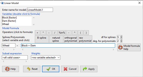
Figure 1. Screenshot Rcmdr Linear Model menu.
then run the ANOVA summary to get the ANOVA table. Rcmdr: Models → Hypothesis tests → ANOVA table.
R Output
Anova Table (Type II tests)

Response: Wheel
           Sum Sq  Df  F value    Pr(>F)
Dam       1467020   3   4.4732   0.01036 *
Block     1672166   2   7.6482   0.00207 **
Residuals 3279544  30
Question 4. Conclusions?
Answer 4. The null hypotheses are:
Treatment factor: Offspring of the different dams have same wheel running activity of offspring.
Blocking factor: No effect of litter parity on wheel running activity of offspring.
Both the treatment factor (p = 0.01036) and the blocking factor (p = 0.00207) were statistically significant.
Questions
Problem 1.
Or we might want to measure the Systolic Blood Pressure of individuals that are on different exercise regimens. However, we are not able to measure all the individuals on the same day at the same time. We suspect that time of day and the day of the year might effect an individuals blood pressure. Given this constraint, the best research design in this circumstance is to measure one individual on each exercise regime at the same time. These different individuals will then be in the same “block” because they share in common the time that their blood pressure was measured. This type of data set would look like this (Table 2):
Table 2. Simulated blood pressure of five subjects on three different exercise regimens.†
|
Subject
|
No
Exercise |
Moderate Exercise
|
Intense Exercise
|
|
1
|
120
|
115
|
114
|
|
2
|
135
|
130
|
131
|
|
3
|
115
|
110
|
109
|
|
4
|
112
|
107
|
106
|
|
5
|
108
|
103
|
102
|
Let’s make a line graph to help us visualize trends (Fig 2).
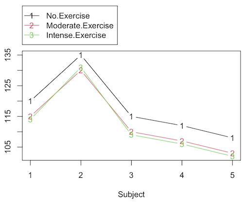
Figure 2. Line graph of data presented in Table 2.
Question 1. Describe the problem and identify the treatment and blocking factors.
Question 2. What is the statistical model?
Question 3. Test the model.
Question 4. Conclusions?
†You’ll need to arrange the data like the data set for the worked example.
Problem 2.
Another example in conservation biology or agriculture. There may be three different management strategies for promoting the recovery of a plant species. A good research design would be to choose many plots of land (blocks) and perform each treatment (management strategy) on a portion of each plot of land (block). A researcher would start with an equal number of plantings in the plots and see how many grew. The plots of land (blocks) share in common many other aspects of that particular plot of land that may effect the recovery of a species.
Table 3. Growth of plants in 5 different plots subjected to one of three management plans (simulated data set).†
|
Plot No.
|
No Management Used
|
Management
Plan 1 |
Management
Plan 2 |
|
1
|
0
|
11
|
14
|
|
2
|
2
|
13
|
15
|
|
3
|
3
|
11
|
19
|
|
4
|
4
|
10
|
16
|
|
5
|
5
|
15
|
12
|
†You’ll need to arrange the data the same arrangement as for the worked example.
These are examples of Two-Factor ANOVA but we are usually only interested in the treatment Factor. We recognize that the blocking factor may contribute to differences among groups and so wish to control for the fact that we carried out the experiments at different times (eg, seasons) or at different locations (eg, agriculture plots)
Question 5. Describe the problem and identify the treatment and blocking factors. Make a line graph to help visualize.
Question 6. What is the statistical model?
Question 7. Test the model.
Question 8. Conclusions?
Repeated-Measures Experimental Design
If multiple measures are taken on the same individual, then we have a repeated-measures experiment. This is a Randomized Block Design. In other words, each animal gets all levels of a treatment (assigned randomly). Thus, samples (individuals) are not independent and the analysis needs to take this into account. Just like for paired-T tests, one can imagine a number of experiments in biomedicine that would conform to this design.
Problem 3.
The data are total blood cholesterol levels for 7 individuals given 3 different drugs (from example given in Zar 1999, Ex 12.5, pp. 257-258).
Table 5. Repeated measures of blood cholesterol levels of seven subjects on three different drug regimens.†
|
Subjects
|
Drug1
|
Drug2
|
Drug3
|
|
1
|
164
|
152
|
178
|
|
2
|
202
|
181
|
222
|
|
3
|
143
|
136
|
132
|
|
4
|
210
|
194
|
216
|
|
5
|
228
|
219
|
245
|
|
6
|
173
|
159
|
182
|
|
7
|
161
|
157
|
165
|
†You’ll need to arrange the data like the data set for the worked example.
Question 9: Is there an interaction term in this design? Make a line graph to help visualize.
Question 10: Are individuals a fixed or a random effect?
Question 11. What is the statistical model?
Question 12. Test the model. Note that we could have done the experiment with 21 randomly selected subjects and a one-factor ANOVA. However, the repeated measures design is best IF there is some association (“correlation”) between the data in each row. The computations are identical to the randomized block analysis.
Question 13. Conclusions?
Problem 4.
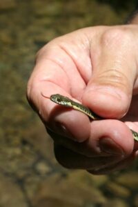
Figure 3. Juvenile garter snake, image from juvenile garter snake in hand, public domain.
Here is a second example of a repeated measures design experiment. Garter snakes (Fig 3) respond to odor cues to find prey. Snakes use their tongues to “taste” the air for chemicals, and flick their tongues rapidly when in contact with suitable prey items, less frequently for items not suitable for prey. In the laboratory, researchers can test how individual snakes respond to different chemical cues by presenting each snake with a swab containing a particular chemical. The researcher then counts how many times the snake flicks its tongue in a certain time period (data presented p. 301, Glover and Mitchell 2016).
Table 6. Tongue flick counts of naïve newborn snakes to extracts†
|
Snake
|
Control (dH2O)
|
Fish mucus
|
Worm mucus
|
|
1
|
3
|
6
|
6
|
|
2
|
0
|
22
|
22
|
|
3
|
0
|
12
|
12
|
|
4
|
5
|
24
|
24
|
|
5
|
1
|
16
|
16
|
|
6
|
2
|
16
|
16
|
†You’ll need to arrange the data like the data set for the worked example.
Question 14. Describe the problem and identify the treatment and blocking factors. Make a line graph to help visualize.
Question 15. What is the statistical model?
Question 16. Test the model.
Question 17. Conclusions?
Quiz Chapter 14.4
Randomized block design
Data sets used in this page
Problem 1 data set
| Block | Dam | Wheel |
|---|---|---|
| B1 | D1 | 1100 |
| B1 | D2 | 1566 |
| B1 | D3 | 945 |
| B1 | D4 | 450 |
| B1 | D1 | 1245 |
| B1 | D2 | 1478 |
| B1 | D3 | 877 |
| B1 | D4 | 501 |
| B1 | D1 | 1115 |
| B1 | D2 | 1502 |
| B1 | D3 | 892 |
| B1 | D4 | 394 |
| B2 | D1 | 999 |
| B2 | D2 | 451 |
| B2 | D3 | 644 |
| B2 | D4 | 605 |
| B2 | D1 | 899 |
| B2 | D2 | 405 |
| B2 | D3 | 650 |
| B2 | D4 | 612 |
| B2 | D1 | 745 |
| B2 | D2 | 344 |
| B2 | D3 | 605 |
| B2 | D4 | 700 |
| B3 | D1 | 1245 |
| B3 | D2 | 702 |
| B3 | D3 | 1712 |
| B3 | D4 | 790 |
| B3 | D1 | 1300 |
| B3 | D2 | 612 |
| B3 | D3 | 1745 |
| B3 | D4 | 850 |
| B3 | D1 | 1750 |
| B3 | D2 | 508 |
| B3 | D3 | 1680 |
| B3 | D4 | 910 |