3.5 – Statistics of error
Making sense of error in data.
This page explains how statistics of error help quantify differences between measured and true values, beginning with classical methods like standard error and confidence intervals that rely on large-sample assumptions. Related, statisticians talk about uncertainty — the quantification of doubt about a measurement. We introduce permutation-based approaches, including jackknife and bootstrap resampling, which avoid those assumptions and are especially useful with smaller or complex data sets. Observer variation (intra- and interobserver error) is also highlighted as an important source of measurement error.
Missing values are another common source of uncertainty in biological data sets. Data may be missing because of equipment failure, recording mistakes, sample loss, or biological factors that prevent a measurement from being collected. Even a small number of missing observations can influence summaries, graphs, and statistical tests, especially in smaller studies. In this chapter, we treat missing values mainly as a practical issue to identify and report during exploratory data analysis. Later, in the chapter on experimental design, we examine missing data in greater depth, including differences between random and non-random missingness, as well as approaches such as data imputation and the consequences these choices may have for interpretation.
We conclude with a discussion about confidence intervals as a measure of accuracy and emphasize proper use of significant figures to avoid overstating precision.
Statistics of error.
In statistics, error doesn’t mean mistake, an avoidable human misjudgement or oversight, eg, a typo. An error in statistics means there was a difference between the measured value and the actual value for an object. Efforts by many authors of notable classical statistics developed a large body of calculated statistics, eg, standard error the mean, which allows the user to quantify how large the error of measurement is given assumptions about the distribution of the errors. Thus, classical statistics requires user to make assumptions about the error distribution, the subject of our Chapter 6. A critical issue to understand is that these methods assume large sample sizes are available; they are called asymptotic statistics or large-sample statistics; the properties of the statistical estimates are evaluated as sample size approaches infinity.
Jackknife sampling and bootstrap sampling are permutation approaches to working with data when the Central Limit Theorem — as sample size increases, the distribution of sample means will tend to a normal distribution (see Chapter 6.7) — is unlikely to apply or, rather, we don’t wish to make that assumption (Chapter 19). The jackknife is a sampling method involving repeatedly sampling from the original data set, but each time leaving one value out. The estimator, for example, the sample mean, is calculated for each sample. The repeated estimates from the jackknife approach yield many estimates which, collected, are used to calculate the sample variance. Jackknife estimators tend to be less biased than those from classical asymptotic statistics.
Bootstrapping, and not jackknife resampling, may now be the preferred permutation approach (eg, Google Scholar search “bootstrap statistics” 36K hits; “jackknife statistics” 17K hits), but which method is best depends on qualities of the data set. Bootstrapping involves large numbers of permutations of the original data, which, in short, means we repeatedly take many samples of our data and recalculate our statistics on these sets of sampled data. We obtain statistical significance by comparing our result from the original data against how often results from our permutations on the resampled data sets exceed the originally observed results. By permutation methods, the goal is to avoid the assumptions made by large-sample statistical inference, ie, reaching conclusions about the population based on samples from the population. Since its introduction, “bootstrapping” has been shown to be superior in many — but, importantly, not all — cases for statistics of error compared to the standard, classical approach (Efron 1979, Hesterberg 2015).
There are many advocates for the permutation approaches, and, because we have computers now instead of the hand calculators our statistics ancestors used, permutation methods may be the approach you will take in your own work. However, the classical approach has its strengths — when the conditions, that is, when the assumptions of asymptotic statistics are met by the data, then the classical approaches tend to be less conservative than the permutation methods. By conservative, statisticians mean that a test performs at the level we expect it to. Thus, if the assumptions of classical statistics are met they return the correct answer more often than do the permutation tests.
Error and the observer.
Individual researchers make observations, therefore, we can talk about observer variation as a kind of error measurement. For repeated measures of the same object by an individual, we would expect the individual to return the same results. To the extent repeated measures differ, this is intraobserver error. In contrast, measures of the same object from different individuals is interobserver error. For a new instrument or measurement system, one would need to establish the reliability of the measure: confronted with the same object do researchers get the same measurement? Accounting for interobserver error applies in many fields, eg, histopathology of putative carcinoma slides (Franc et al 2003), liver biopsies for cirrhosis (Rousselet et al 2005), blood cell counts (Bacus 1973).
Confidence in estimates.
A really useful concept in statistics is the idea that you can assign how confident you are to an estimate. This is another way to speak of the accuracy of an estimate. Clearly, we have more confidence in a sample estimate for a population parameter if many observations are made. Another factor in our ability to estimate is the magnitude of observation differences. In general, the larger the differences among values from repeated trials, the less confident we will be in out estimate, unless, again, we make our estimates from a large collection of observations. These two quantities, sample size and variability, along with our level of confidence, eg, 95%, are incorporated into a statistic called the confidence interval.

We will use this concept a lot throughout the course; for now, a simple but approximate confidence interval is to use the 2 x SEM rule (as long as sample size large): twice the standard error of the mean. Take your estimate of the mean, then add (upper limit) or subtract (lower limit) twice the value of the standard error of the mean (if you recall, that’s the standard deviation divided by the square-root of the sample size).
Example. Consider five magnetic darts thrown at a dart board (28 cm diameter, height of 1.68m from the floor) from a distance of 3.15 meters (Fig 1).

Figure 1. Magnetic dart board with 5 darts. Click image to view full sized image.
The distance in centimeters (cm) between where each of the five darts landed on the board compared to the bullseye is reported in (Table 1),
Table 1. Results of five darts thrown at a target (Figure 2)*
| Dart | Distance |
|---|---|
| 1 | 7.5 |
| 2 | 3.0 |
| 3 | 1.0 |
| 4 | 2.7 |
| 5 | 7.4 |
* distance in centimeters from the center.
Note 1: Use of the coordinate plane, and including the angle measurement in addition to distance (the vector) from center, would be a better analysis. In the context of darts, determining accuracy of a thrower is an Aim-Point targeting problem and part of your calculation would be to get MOA (minute of angle). For the record, the angles (degrees) were
| Dart | Distance | Angle |
|---|---|---|
| 1 | 7.5 | 124.4 |
| 2 | 3.0 | -123.7 |
| 3 | 1.0 | 96.3 |
| 4 | 2.7 | -84.3 |
| 5 | 7.4 | -31.5 |
measured using imageJ. Because there seems to be an R package for just about every data analysis scenario, unsurprisingly, there’s an R package called shotGroups to analyze shooting data.
How precise was the dart thrower? We’ll use the coefficient of variation as a measure of precision. Second, how accurate were the throws? Use R to calculate
darts = c(7.5, 3.0, 1.0, 2.7, 7.4)
#use the coefficient of variation to describe precision of the throws
coefVar = 100*(sd(darts)/mean(darts)); coefVar
[1] 68.46141
Confidence Interval to describe accuracy.
For a game of darts, the true value would be a distance of zero — all bullseyes. We need to calculate the standard error of the mean (SEM), then, we calculate the confidence interval around the sample mean.
#Calculate the SEM
SEM <- sd(darts)/sqrt(length(darts)); SEM
[1] 1.322649
#now, get the lower and upper limit, subtract from the mean
confidence <- c(mean(darts)-2*SEM, mean(darts), mean(darts)+2*SEM); confidence
[1] 1.674702, 4.320000, 6.965298
The mean was 4.3 cm, therefore to get the lower limit of the interval subtract 2.65 (2*SEM = 2.645298) from the mean; for the upper limit add 2.65 to the mean. Thus, we report our approximate confidence interval as (1.7, 7.0), and we read this as saying we are about 95% confident the population value is between these two limits. Five is a very small sample number, so we shouldn’t be surprised to learn that our approximate confidence interval would be less than adequate. In statistical terms, we would use the t-distribution, and not the normal distribution, to make our confidence interval in cases like this.
Note 2: As a rule, implied by Central Limit theory and use of asymptotic statistical estimation, a sample size of 30 or more is safer, but probably unrealistic for many experiments. This is sometimes called as the rule of thirty. (For example, a 96-well PCR array costs about $500; with n = 30, that’s $15,000 US Dollars for one group!). So, what about this rule? This type of thinking should be avoided as “a relic of the pre-computer era,” (Hesterberg, T. (2008). It’s Time To Retire the” n>= 30″ rule.). We can improve on asymptotic statistics by applying bootstrap principles (Chapter 19).
We made a quick calculation of the confidence interval; we can get make this calculation by hand by incorporating the t distribution. We need to know the degrees of freedom, which in this case is 4 (n – 1, where n = 5). We look up critical value of t at 5% (to get our 95% confidence interval), t = 2.78. Subtract for lower limit t*SEM and add for upper limit t*SEM to the sample mean for the 95% confidence interval.
We can get help from R, by using the one-sample t-test with a test against the hypothesis that the true mean is equal to zero. Among a variety of output we will introduce later (see Chapter 8 and 10), the confidence interval is reported (yellow highlight),
#make an attach a data frame object
Ddarts <- data.frame(darts)
t.test(darts,mu=0)
One Sample t-test
data: darts
t = 3.2662, df = 4, p-value = 0.0309
alternative hypothesis: true mean is not equal to 0
95 percent confidence interval:
 0.6477381 7.9922619
sample estimates:
mean of x
 4.32
t.test uses the function qt(), which provides the quantile function. To recreate the 95% CI without the additional baggage output from the t.test, we would simply write
#upper limit
mean(darts)+ qt(0.975,df=4)*sd(darts)/sqrt(5)

#lower limit
mean(darts)+ qt(0.025, df = 4, lower.tail=TRUE)*sd(darts)/sqrt(5)
where sd(darts)/sqrt(5) is the standard error of the mean.
Or, alternatively, download and take advantage of a small package called Rmisc (not to be confused with the RcmdrMisc package) and use the function CI
library(Rmisc)
CI(darts)
     upper     mean     lower
7.9922619 4.3200000 0.6477381
The advantage of using the CI() command from the package Rmisc is pretty clear; I don’t have to specify the degrees of freedom or the standard error of the mean. By default, CI reports the 95% confidence interval. we can specify any interval simply by adding to the command. For example,
CI(darts, ci=0.90)
reports upper and lower limits for the 90% confidence interval.
Try it. On your own, get the 90% confidence interval and the 99% confidence intervals for our dart example. Compare to the 95% confidence interval — what do you conclude about “confidence” in our estimate from 90% to 99%?
Confidence intervals from p-values.
And finally, it is not unusual for a report to provide summary statistics, differences between means (ie, effect size), and p-values (orange highlight), but not report confidence intervals. We discuss p-values and the concept of statistical significance beginning in Chapter 8. But for now, we show how to calculate approximate confidence intervals from the p-value. This may be of use for conducting meta-analysis (Chapter 20.15). See two helpful “how to” articles by Bland and Altman in 2011 BMJ (references listed in Chapter 3.6 – References).
In brief, calculate the test statistic for a normal distribution (letZ), calculate a standard error, and then the lower and upper limits for the 95% confidence interval. We illustrate use of the calculator formulas with the dart example, the p-value was 0.0309; the estimate was 4.32.
R code
letZ = (-0.862 + sqrt(0.743 - 2.404*log(0.0309, base = exp(1)))) = 2.154903
letSE = 4.32/letZ = 2.00473
1.96*letSE = 3.929271 # Add for upper and subtract for lower
The lower limit is 0.39 (4.32 – 3.929271) and the upper limit is 8.25 (4.32 + 3.929271). Although in the ballpark, these calculated estimates are wider than the confidence interval estimated by the t.test command. Small sample size, n = 5, is to blame — the accuracy of these methods, based on asymptotic statistical estimation approaches, assumes the law of large numbers applies.
Significant figures.
And finally, we should respect significant figures, the number of digits which have meaning. Our data were measured to the nearest tenth of a centimeter, or two significant figures. Therefore, if we report the confidence interval as (0.6477381, 7.9922619), then we imply a false level of precision, unless we also report our random sampling error of measurement.
R has a number of ways to manage output. One option would be to set number of figures globally with the options() function — all values reported by R would hold for the entire session. For example, options(digits=3) would report all numbers to three significant figures. Instead, I prefer to use signif() function, which allows us to report just the values we wish and does not change reporting behavior for the entire session.
signif(CI(darts),2)
upper  mean lower
 8.00  4.30  0.65
Note 3: The options() function allows the R user to set a number of settings for an R session. After gaining familiarity with R, the advanced user recognizes that many settings can be changed to make the session work to report in ways more convenient to the user. If curious, submit options() at the R prompt and available settings will be displayed.
The R function signif() applies rounding rules. We apply rounding rules when required to report estimates to appropriate levels of precision. Rounding procedures are used to replace a number with a simplified approximation. Wikipedia provides a comprehensive list of rounding rules. Notable rules include
- directed rounding to an integer, eg, rounding up or down
- rounding to nearest integer, eg, round half up (down) if the number ends with 5
- randomly rounding to an integer, eg, stochastic rounding.
With the exception of stochastic rounding, all rounding methods impose biases on the sets of numbers. For example, the round half up method applied for numbers above 5, round down for numbers below 5 will increase the variance of the sample. In R, use round() for most of your work. If you need one of the other approaches, for example, to round up, the command is ceiling(); to round down we use floor().
When to round?
No doubt your previous math classes have cautioned you about the problems of rounding error and their influence on calculation. So, as a reminder, if reporting calls for rounding, then always round after you’ve completed your calculations, never during the calculations themselves.
A final note about significant figures and rounding. While the recommendations about reporting statistics are easy to come by (and often very proscriptive, eg, Table 1, Cole 2015), there are other concerns. Meta-analysis, which are done by collecting information from multiple studies, would benefit if more and not fewer numbers are reported, for the very same reason that we don’t round during calculations.
Questions
- Calculate the correct 90% and 99% confidence intervals for the dart data using the t-distribution
- by hand
- by one alternative method in R, demonstrated with examples in this page
- How many significant figures should be used for the volumetric pipettor p1000? The p200? The p20 (data at end of this page)?
- Another function,
round(), can be used. Try
round(CI(darts),2)
-
- and report the results: vary the significant figures from 1 to 10 (
signif()will take digits up to 22). - See any output differences between
signif()andround()? Don’t forget to take advantage of R help pages (eg, enter?roundat the R prompt) and see Wikipedia.
- and report the results: vary the significant figures from 1 to 10 (
- Compare rounding by
signif()andround()for the number 0.12345. Can you tell which rounding method the two functions use? - Calculate the coefficient of variation (CV) for each of the three volumetric pipettors from the data at end of this page. Rank the CV from smallest to largest. Which pipettor had the smallest CV and would therefore be judged the most precise?
- (data provided at end of this page, click here).
- Standards distinguish between within run precision and between run precision of a measurement instrument (see Chapter 16.5 – Instrument reliability and validity). The data in Table 1 were all recorded within 15 minutes by one operator. What kind pf precision was measured?
- Calculate the standard error of the means for each of the three pipettors from the data
- (data provided at end of this page, click here).
- Calculate the approximate confidence interval using the 2SE rule and judge which of the three pipettors is the most accurate (narrowest confidence interval)
- Repeat, but this time apply your preferred R method for obtaining confidence intervals.
- Compare approximate and R method confidence intervals. How well did the approximate method work?
- Return to the dart example, but now assume the p-value was p = 0.003 and again for p = 0.0003. Estimate the 95% confidence interval for each case; the difference remains 4.32. How does the change in p-value, from 0.03 to 0.0003 — a two orders of magnitude difference — affect the estimates for the confidence interval (hint: describe the width of the CI)?
Quiz Chapter 3.5
Statistics of error
Data sets
Pipette calibration
| p1000 | p200 | p100 |
|---|---|---|
| 0.113 | 0.1 | 0.101 |
| 0.114 | 0.1 | 0.1 |
| 0.113 | 0.1 | 0.1 |
| 0.115 | 0.099 | 0.101 |
| 0.113 | 0.1 | 0.101 |
| 0.112 | 0.1 | 0.1 |
| 0.113 | 0.1 | 0.1 |
| 0.111 | 0.1 | 0.1 |
| 0.114 | 0.101 | 0.101 |
| 0.112 | 0.1 | 0.1 |
Chapter 3 continues
16.1 – Product moment correlation
Introduction.
A correlation is used to describe the direction  magnitude of linear association and the between two variables. There are many types of correlations, some are based on ranks, but the one most commonly used is the product-moment correlation (r). The Pearson product-moment correlation is used to describe association between continuous, ratio-scale data, where “Pearson” is in honor of Karl Pearson (b 1857 – d. 1936).
There are many other correlations, including Spearman’s and Kendall’s tau (τ) (Chapter 16.4) and ICC, the intraclass correlation (Chapter 12.3 and Chapter 16.4).
The product moment correlation is appropriate for variables of the same kind — for example, two measures of size, like the correlation between body weight and brain weight.
Spearman’s and Kendall’s tau correlation are nonparametric and would be alternatives to the product moment correlation. The intraclass correlation, or ICC, is a parametric estimate suitable for repeat measures of the same variable.
The correlation coefficient.

The numerator is the sum of products and it quantifies how the deviates from X and Y means covary together, or change together. The numerator is known as a “covariance.”

The denominator includes the standard deviations of X and Y; thus, the correlation coefficient is the standardized covariance.
The product moment correlation, r, is an estimate of the population correlation, ρ (pronounced rho), the true relationship between the two variables.
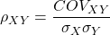
where COV(X,Y) refers to the covariance between X and Y.
Effect size.
Estimates for r range from -1 to +1; the correlation coefficient has no units. A value of 0 describes the case of no statistical correlation, ie, no linear association between the two variables. Usually, this is taken as the null hypothesis for correlation — “No correlation between two variables,” with the alternative hypothesis (2-tailed) — “There is a correlation between two variables.”
Like mean difference effect size, we can report the strength of correlation between two variables. Consider the magnitude and not the direction . Like Cohen’s effect size:
| Absolute value | Magnitude of association |
| 0.10 | small, weak |
| 0.30 | moderate |
| > 0.50 | strong, large |
Note that one should not interpret a “strong, large” correlation as evidence that the association is necessarily real. See Ch16.c for more on spurious correlations.
Standard error of the correlation.
An approximate standard error for r can be obtained using this simple formula
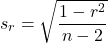
This standard error can be used for significance testing with the t-test. See below.
Confidence interval.
Like all situations in which an estimate is made, you should report the confidence interval for r. The standard error approximation is appropriate when the hull hypothesis is  , because the joint distribution is approximately normal. However, as the estimate approaches the limits of the closed interval
 , the distribution becomes increasingly skewed.
The approximate confidence interval for the correlation is based on Fisher’s z-transformation. We use this transformation to stabilize the variance over the range of possible values of the correlation and, therefore, better meet the assumptions of parametric tests based on the normal distribution.
The transform is given by the equation
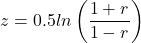
where ln is the natural logarithm. In the R language we get the natural log by log(x), where x is a variable we wish to transform.
Equivalently, z can be rewritten as

the inverse hyperbolic tangent function. In R language this function is called by atanh(r) at the R prompt.
The standard error for z is about
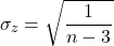
We take z to be the estimate of the population zeta, ζ. We take the sampling distribution of z to be approximately normal and thus we may then use the normal table to generate the 95% confidence interval for zeta.

Why 1.96? We want 95% confidence interval, so that at Type I α = 0.05, we want the two tails of the Normal distribution (see Appendix 20.1), or + 0.025. Thus +0.025 is +1.96 and -1.96 corresponds to 0.025 (α = 0.05/2 tails = 0.025).
Significance testing.
Significance testing of correlations is straightforward, with the noted caveat about the need to transform in cases where the estimate is close to  . For the typical test of null hypothesis, the correlation, r, is equal to 0, the t distribution can be used (ie, it’s a t-test).

which has degrees of freedom, DF = n – 2.
Use the t-table critical values to test the null hypothesis involving product moment correlation (eg, Appendix 20.3; for Spearman rank correlation  , see Table G, p. 686 in Whitlock & Schluter).
Alternatively (and preferred), we’ll just use R and Rcmdr’s facilities without explanation; the t distribution works OK as long as the correlations are not close to , in which case other things need to be done — and this is also true if you want to calculate a confidence interval for the correlation.
You are sufficiently skilled at this point to evaluate whether a correlation is statistically significantly different from zero — just check out whether the associated P-value is less than or greater than alpha (usually set at 5%). A test of whether or not the correlation, r1, is equal to some value, r2, other than zero is also possible. For an approximate test, replace zero in the above test statistic calculation with the value for r2, and calculate the standard error of the difference. Note that use of the t-test for significance testing of the correlation is an approximate test — if the correlations are small in magnitude using the Fisher’s Z transformation approach will be less biased, where the test statistic z now is

and standard error of the difference is

and look up the critical value of z from the normal table.
R code.
To calculate correlations in R and Rcmdr, have ratio-scale data ready in the columns of a R and Rcmdr data frame. We’ll introduce the commands with an example data set from my genetics laboratory course.
Question. What is the estimate of the product moment correlation between Drosophila fly wing length and area?
Data (thanks to some of my genetics students!)
Area <- c(0.446, 0.876, 0.390, 0.510, 0.736, 0.453, 0.882, 0.394, 0.503, 0.535, 0.441, 0.889, 0.391, 0.514, 0.546, 0.453, 0.882, 0.394, 0.503, 0.535)
Length <- c(1.524, 2.202, 1.520, 1.620, 1.710, 1.551, 2.228, 1.460, 1.659, 1.719, 1.534, 2.223, 1.490, 1.633, 1.704, 1.551, 2.228, 1.468, 1.659, 1.719)
Create your data frame, eg,
FlyWings <- data.frame(Area, Length)
And here’s the scatterplot (Fig 1). We can clearly see that Wing Length and Wing Area are positively correlated, with one outlier (Fig 1).
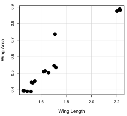
Figure 1. Scatterplot of Drosophila wing area by wing length.
The R command for correlation is simply cor(x,y). This gives the “pearson” product moment correlation, the default. To specify other correlations, use method = "kendall", or method = "spearman" (See Chapter 16.4).
Question. What are the Pearson, Spearman, and Kendall’s tau estimates for the correlation between fly Wing Length and Wing Area?
At the R prompt, type
cor(Length,Area)
[1] 0.9693334
cor(Length,Area, method="kendall")
[1] 0.8248008
cor(Length,Area, method="spearman")
[1] 0.9558658
Note that we entered Length first. On your own, confirm that the order of entry does not change the correlation estimate. To both estimate test the significance of the correlation between Wing Area and Wing Length, at the R prompt type
cor.test(Area, Length, alternative="two.sided", method="pearson")
R returns with
Pearson's product-moment correlation

data: Area and Length

t = 16.735, df = 18, p-value = 2.038e-12>
alternative hypothesis: true correlation is not equal to 0
95 percent confidence interval:
0.9225336 0.9880360
sample estimates:
   cor
0.9693334
Alternatively, to calculate and test the correlation, use R Commander, Rcmdr: Statistics → Summaries→ Correlation test
Note 1. R’s cor.test uses Fisher’s z transformation; note if we instead use the approximate calculation instead how poor the approximation works in this example. The estimated correlation was 0.97, thus the approximate standard error was 0.058. The confidence interval (t-distribution, alpha=0.05/2 and 18 degrees of freedom) was between 0.848 and 1.091, which is greater than the z transform result and returns an out-of-bounds upper limit.
Alternative packages to base R provide more flexibility and access to additional approaches to significance testing of correlations (Goertzen and Cribbie 2010). For example, z_cor_test() from the TOSTER package.
z_cor_test(Area, Length)

Pearson's product-moment correlation
data:  Area and Length
z = 8.5808, N = 20, p-value < 2.2e-16
alternative hypothesis: true correlation is not equal to 0
95 percent confidence interval:
0.9225336 0.9880360
sample estimates:
      cor
0.9693334
To confirm, check the critical value for z = 8.5808, two-tailed, with
> 2*pnorm(c(8.5808), mean=0, sd=1, lower.tail=FALSE)
[1] 9.421557e-18
Note the difference is that Fisher’s z is used for hypothesis testing; cor.test and z_cor_test return same confidence intervals.
and by bootstrap resampling (see Chapter 19.2),
boot_cor_test(Area, Length)

Bootstrapped Pearson's product-moment correlation

data: Area and Length
N = 20, p-value < 2.2e-16
alternative hypothesis: true correlation is not equal to 0
95 percent confidence interval:
0.8854133 0.9984744
sample estimates:
cor
0.9693334
The z-transform confidence interval would be preferred over the bootstrap confidence interval because it is narrower.
Assumptions of the product-moment correlation.
Interestingly enough, there are no assumptions for estimating a statistic. You can always calculate an estimate, although of course, this does not mean that you have selected the best calculation to describe the phenomenon in question, it just means that assumptions are not applicable for estimation. Whether it is the sample mean or the correlation, it is important to appreciate that, look, you can always calculate it, even if it is not appropriate!
Statistical assumptions and those technical hypotheses we evaluate apply to statistical inference — being able to correctly interpret a test of statistical significance for a correlation estimate depends on how well assumptions are met. The most important assumption for a null hypothesis test of correlation is that samples were obtained from a “bivariate normal distribution.” It is generally sufficient to just test normality of the variables one at a time (univariate normality), but the student should be aware that testing the bivariate normality assumption can be done directly (eg, Doornick and Hansen 2008).
Testing two independent correlations
Extending from a null hypothesis of the correlation is equal to zero to the correlation equals a particular value should not be a stretch for you. For example, since we use the t-test to evaluate the null hypothesis that the correlation is equal to zero, you should be able to make the connection that, like the two sample t-test, we can extend the test of correlation to any value. However, using the t-test without considering the need to stabilize the variance.
When two correlations come from independent samples, we can test whether or not the two correlations are equal. Rather than use the t-test, however, we use a modification of Fisher’s Z transformation. Calculate z for each correlation separately, then use the following equation to obtain Z. We then look up Z from our table of standard normal distribution (Appendix 20.1, or better — use the normal distribution functions in Rcmdr) and we can obtain the p-value of the test of the hypothesis that the two correlations are equal.
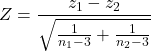
Example. Two independent correlations are r1 = 0.2 and r2 = 0.34. Sample sizes for group 1 was 14 and for group 2 was 21. Test the hypothesis that the two correlations are equal. Using R as a calculator, here’s what we might write in the R script window and the resulting output. It doesn’t matter which correlation we set as r1 or r2, so I prefer to calculate the absolute value of Z and then get the probability from the normal table for values greater or equal to |Z| (ie, the upper tail).
z1 = atanh(0.2)
z2 = atanh(0.34)
n1 = 14
n2 = 21
Z = abs((z1-z2)/sqrt((1/(n1-3))+(1/(n2-3))))
Z = 0.3954983
From the normal distribution table we get a p-value of 0.3462 for the upper tail. Because this p-value is not less than our typical Type I error rate of 0.05, we conclude that the two correlations are not in fact significantly different.
Rcmdr: Distributions → Continuous distributions → Normal distribution → Normal probabilities…
pnorm(c(0.3954983), mean=0, sd=1, lower.tail=FALSE)
R returns
[1] 0.3462376
To make this two-tailed, of course all we have to do is multiple the one-tailed p-value by two, in this case two-tailed p-value = 0.69247.
Write a function in R
There’s nothing wrong with running the calculations as written. But R allows users to write their own functions. Here’s one possible function we could write to test two independent correlations. Write the R function in the script window.
test2Corr = function(r1,r2,n1,n2) {
z1=atanh(r1); z2=atanh(r2)
Z = abs((z1-z2)/sqrt((1/(n1-3))+(1/(n2-3))))
pnorm(c(Z), mean=0, sd=1, lower.tail=FALSE)
}
After submitting the function, we then invoke the function by typing at the R prompt
p = test2Corr(0.2,0.34,14,21); p
Again, R returns the one-tailed p-value
[1] 0.3462376
Unsurprisingly, these simple functions are often available in an R package. In this case, the psych package provides a function called r.test() which will accommodate the test of the equality hypothesis of two independent correlations. Assuming that the psych package has been installed, at the R prompt we type
require(psych)
r.test(14,.2,.34,n2=21,twotailed=TRUE)
And R returns
Correlation tests
Call:r.test(n = 14, r12 = 0.20, r34 = 0.34, n2 = 21, twotailed = TRUE)
Test of difference between two independent correlations
z value 0.4 with probability 0.69
More on testing correlations
The discussion above, as stated, assumes the two correlations are independent of each other. In ecological studies, for example, it is not uncommon to have estimates for correlations among multiple pairs of traits. Thus, our approach would not be appropriate for testing whether the difference in correlations between body mass/ornament size and body mass/swimming performance of male killifish because both correlations include the same variable (body mass). A better solution would be to use William’s t-test (Williams 1959, Diedenhofen and Musch 2015).
Note 2: This example was selected from Sowersby et al 2022 — I’m not implying here that the authors analyzed their results incorrectly, I just like the example of traits to illustrate the point!
The null hypothesis was evaluated using Williams’ (1959)  -test for overlapping dependent correlations with
 degrees of freedom, calculated as:
(1) 
Where  represents the determinant of the
 correlation matrix, defined as:
(2) 
The r.test() in psyche package can be modified to handle this. R code for a made up example:
# 1. Define your sample size (N)
sample_size <- 65 # Example: 65 male killifish

# 2. Define the three correlation coefficients (r)
# r12 = correlation between body mass and ornament size
# r13 = correlation between body mass and swimming performance
# r23 = correlation between ornament size and swimming performance
r_mass_ornament <- 0.55
r_mass_swim <- 0.30
r_ornament_swim <- 0.40

# 3. Run Williams' t-test using r.test()
result <- psych::r.test(
   n = sample_size,
   r12 = r_mass_ornament,
   r13 = r_mass_swim,
  r23 = r_ornament_swim
)

# 4. View the results
print(result)
R output
Correlation tests
Call:[1] "r.test(n = 65 , r12 = 0.55 , r23 = 0.4 , r13 = 0.3 )"
Test of difference between two correlated correlations
t value 2.13 with probability < 0.037NULL
And we would conclude that the two correlations are indeed statistically different from each other.
Alternatively, use the cocor.dep.groups.overlap() from the cocor package. This generates all of the proposed tests of such correlations.
For our example then,
library(cocor)

# 1. Define sample size (N)
sample_size <- 65
# 2. Define individual correlations (r)
# r.jk = correlation between body mass (j) and ornament size (k)
# r.jh = correlation between body mass (j) and swimming performance (h)
# r.kh = correlation between ornament size (k) and swimming performance (h)
r_mass_ornament <- 0.55
r_mass_swim <- 0.30
r_ornament_swim <- 0.40
#3. Note: j is the overlapping/shared variable (body mass)
my_result <- cocor.dep.groups.overlap(
    r.jk = r_mass_ornament,
    r.jh = r_mass_swim,
   r.kh = r_ornament_swim,
   n = sample_size,
   alternative = "two.sided",
   alpha = 0.05
)

# 4. View the full comparison report
show(my_result)
Note 3: To extract and print ONLY Williams’ t-test results use my_results@williams1959.
R output (rearranged, brought William’s t-test up to the top for comparisons).
Results of a comparison of two overlapping correlations based on dependent groups

Comparison between r.jk = 0.55 and r.jh = 0.3
Difference: r.jk - r.jh = 0.25
Related correlation: r.kh = 0.4
Group size: n = 65
Null hypothesis: r.jk is equal to r.jh
Alternative hypothesis: r.jk is not equal to r.jh (two-sided)
Alpha: 0.05

williams1959: Williams' t (1959)
t = 2.1291, df = 62, p-value = 0.0372
Null hypothesis rejected

pearson1898: Pearson and Filon's z (1898)
z = 2.1217, p-value = 0.0339
Null hypothesis rejected

hotelling1940: Hotelling's t (1940)
t = 2.1635, df = 62, p-value = 0.0344
Null hypothesis rejected

olkin1967: Olkin's z (1967)
z = 2.1217, p-value = 0.0339
Null hypothesis rejected

dunn1969: Dunn and Clark's z (1969)
z = 2.0926, p-value = 0.0364
Null hypothesis rejected

hendrickson1970: Hendrickson, Stanley, and Hills' (1970) modification of Williams' t (1959)
t = 2.1635, df = 62, p-value = 0.0344
Null hypothesis rejected

steiger1980: Steiger's (1980) modification of Dunn and Clark's z (1969) using average correlations
z = 2.0795, p-value = 0.0376
Null hypothesis rejected

meng1992: Meng, Rosenthal, and Rubin's z (1992)
z = 2.0675, p-value = 0.0387
Null hypothesis rejected
95% confidence interval for r.jk - r.jh: 0.0161 0.6017
Null hypothesis rejected (Interval does not include 0)

hittner2003: Hittner, May, and Silver's (2003) modification of Dunn and Clark's z (1969) using a backtransformed average Fisher's (1921) Z procedure
z = 2.0741, p-value = 0.0381
Null hypothesis rejected

zou2007: Zou's (2007) confidence interval
95% confidence interval for r.jk - r.jh: 0.0155 0.4877
Null hypothesis rejected (Interval does not include 0)
Note 4: show() not summary() because cocor.dep.groups.overlap() returns an S4 object.
Questions
- Write up three learning outcomes for this page. Hint: Point your favorite generative AI to this page and ask for help.
- True or False. Generally, the null hypothesis of a test of a correlation is Ho: r = 0, although in practice, one could test a null of r = any value.
- Return to the fly wing example. What was the estimate of the value of the product moment correlation? The Spearman Rank correlation? The Kendall’s tau?
- OK, you have three correlation estimates for test of the same null hypothesis, ie, correlation between Length and Area is zero. Which estimate is the best estimate?
- Apply the Fisher z transformation to the estimated correlation, what did you get?
- For the fly wing example, what were the degrees of freedom?
- For the fly wing example, calculate the approximate standard error of the product moment correlation.
- Return one last time to the fly wing example. What was the value of the lower limit of the 95% confidence interval for the estimate of the product moment correlation? And the value of the upper limit?
- Assume that another group of students (n = 15) made measurements on fly wings and the correlation was 0.86. Is the difference between the two correlations for the two groups of students equal? Obtain the probability using the Z calculation and R (Chapter 6.7) or the normal table.
Quiz Chapter 16.1
Product moment correlation
Chapter 16 contents
12.3 – Fixed effects, random effects, and agreement
Introduction
Within discussions of one-way ANOVA models the distinction between two general classes of models needs to be made clear by the researcher. The distinction lies in how the levels of the factor are selected. If the researcher selects the levels, then the model is a Fixed Effects Model, also called a Model I ANOVA. On the other hand, if the levels of the factor were selected by random sampling from all possible levels of the factor, then the model is a Random Effects Model, also called a Model II ANOVA. This page is about such models and I’ll introduce the intraclass correlation coefficient, abbreviated as ICC, as a way to illustrate applications of Model II ANOVA.
Here’s an example to help the distinction. Consider an experiment to see if over the counter painkillers are as good as prescription pain relievers at reducing numbers of migraines over a six week period. The researcher selects Tylenol®, Advil®, Bayer® Aspirin, and Sumatriptan (Imitrex®), the latter an example of a medicine only available by prescription. This is clearly an example of fixed effects; the researcher selected the particular medicines for use.
Random effects, in contrast, implies that the researcher draws up a list of all over the counter pain relievers and draws at random three medicines; the researcher would also randomly select from a list of all available prescription medicines.
Fixed effects are probably the more common experimental approaches. To be complete, there is a third class of ANOVA called a Mixed Model or Model III ANOVA, but this type of model only applies to multidimensional ANOVA (eg, two-way ANOVA or higher), and we reserve our discussion of the Model III until we discuss multidimensional ANOVA (Table 1).
Table 1. ANOVA models
| ANOVA model | Treatments are |
| I | Fixed effects |
| II | Random effects |
| III | Mixed, both fixed & random effects |
Although the calculations for the one-way ANOVA under Model I or Model II are the same, the interpretation of the statistical significance is different between the two.
In Model I ANOVA, any statistical difference applies to the differences among the levels selected, but cannot be generalized back to the population. In contrast, statistical significance of the Factor variable in Model II ANOVA cannot be interpreted as specific differences among the levels of the treatment factor, but instead, apply to the population of levels of the factor. In short, Model I ANOVA results apply only to the study, whereas Model II ANOVA results may be interpreted as general effects, applicable to the population.
This distinction between fixed effects and random effects can be confusing, but it has broad implications for how we interpret our results in the short-term. This conceptual distinction between how the levels of the factor are selected also has general implications for our ability to acquire generalizable knowledge by meta-analysis techniques (Hunter and Schmidt 2000). Often we wish to generalize our results: we can do so only if the levels of the factor were randomly selected in the first place from all possible levels of the factor. In reality, this may not often be the case. It is not difficult to find examples in the published literature in which the experimental design is clearly fixed effects (ie, the researcher selected the treatment levels for a reason), and yet in the discussion of the statistical results, the researcher will lapse into generalizations.
Random Effects Models and agreement
Model II ANOVA is common in settings in which individuals are measured more than once. For example, in behavioral science or in sports science, subjects are typically measured for the response variable more than once over a course of several trials. Another common setting of Model II ANOVA is where more than one raters are judging an event or even a science project. In all of these cases what we are asking is about whether or not the subjects are consistent, in other words, we are asking about the precision of the instrument or measure.
In the assessment of learning by students, for example, different approaches may be tried and the instructor may wish to investigate whether the interventions can explain changes in test scores. To assess instrument validity — an item score from a grading rubric (Goertzen and Klaus 2023), tumor budding as biomarker for colorectal cancer (Bokhorst et al 2020) — agreement or concordance among two or more raters or judges (inter-rater reliability) needs to be established (same citations and references therein). For binomial data, we would be tempted to use the phi coefficient, Is it actually reliable Cohen’s kappa (two judges) or Fleiss Kappa (two or more judges) is a better tool. Phi coefficient and both assessment scores were introduced in Chapter 9.2.
For ratio scale data, agreement among scores of two or more scores from judges There is an enormous number of articles on reliability measures in the social sciences and you should be aware of a classical paper on reliability by Shrout and Fleiss (1979) (see also McGraw and Wong, 1996). Both the ICC and the Pearson product moment correlation, r, which we will introduce in Chapter 16, are measures of strength of linear association between two ratio scale variables (Jinyuan et al 2016). But ICC is more appropriate for association between repeat measures of the same thing, eg, repeat measures of running speed or agreement between judges. In contrast, the product moment correlation can be used to describe association between any two variables, eg, between repeat measures of running speed, but also between say running speed and maximum jumping height. The concept of repeatability of individual behavior or other characteristics is also a common theme in genetics and so you should not be surprised to learn that the concept actually traces to RA Fisher and his invention of ANOVA. Just as in the case of the sociology literature, there are many papers on the use and interpretation of repeatability in the evolutionary biology literature (eg, Lessels and Boag 1987; Boake 1989; Falconer and Mackay 1996; Dohm 2002; Wolak et al 2012).
Agreement and repeatability are Model II (random effects) because the subjects, items, or raters being studied are treated as a random sample from a larger population rather than specific, fixed levels of interest. In reliability studies, subjects are not chosen for their specific characteristics but as representatives of the population variability. The goal is to infer whether a measurement tool works for any future subject or rater, not just the ones tested in the study. These factors are designed to estimate variance components and generalize results beyond the specific sample used. Put another way, the goal of Model II is often to estimate how much variance is due to differences between subjects versus within subjects (repeatability), which requires treating the subject effect as random.
There are many ways to analyze these kinds of data but a good way is to treat this problem as a one-way ANOVA with Random Effects. Thus, the Random Effects model permits the partitioning of the variation in the study into two portions: the amount that is due to differences among the subjects or judges or intervention versus the amount that is due to variation within the subjects themselves. The Factor is the Subjects and the levels of the factor are how ever many subjects are measured twice or more for the response variable.
If the subjects performance is repeatable, then the Mean Square Between (Among) Subjects,  , component will be greater than the Mean Square Error component,
 , of the model. There are many measures of repeatability or reliability, but the intraclass correlation coefficient or ICC is one of the most common. The ICC may be calculated from the Mean Squares gathered from a Random Effects one-way ANOVA. ICC can take any value between zero and one.
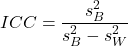
where
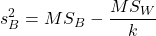
and

B and W refers to the among group (between or among groups mean square) and the within group components of variation (error mean square), respectively, from the ANOVA, MS refers to the Mean Squares, and k is the number of repeat measures for each experimental unit. In this formulation k is assumed to be the same for each subject.
By example, when a collection of sprinters run a race, if they ran it again, would the outcome be the same, or at least predictable? If the race is run over and over again and the runners cross the finish lines at different times each race, then much of the variation in performance times will be due to race differences largely independent of any performance abilities of the runners themselves and the Mean Square Error term will be large and the Between subjects Mean Square will be small. In contrast, if the race order is preserved race after race: Jenny is 1st, Ellen is 2nd, Michael is third, and so on, race after race, then differences in performance are largely due to individual differences. In this case, the Between-subjects Mean Square will be large as will the ICC, whereas the Mean Square for Error will be small, and so will the ICC.
Can the intraclass correlation be negative?
In theory, no. Values for ICC range between zero and one. The familiar Pearson product moment correlation, Chapter 16, takes any value between -1 and +1. However, in practice, negative values for ICC will result if  .
In other words, if the within group variability is greater than the among group variability, then negative ICC are possible. The question is whether negative estimates are ever biologically relevant or, simply result of limitations of the estimation procedure. Small ICC values and few repeats increases the risk of negative ICC estimates. Thus, a negative ICC would be “simply a(n) “unfortunate” estimate (Liljequist et al 2019). However, there may be situations in which negative ICC is more than unfortunate. For example, repeatability, a quantitative genetics concept (Falconer and Mackay 1996), can be negative (Nakagawa and Schielzeth 2010).
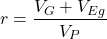
Repeatability reflects the consistency of individual traits over time (or spatially, eg, scales on on a snake), is defined as the ratio of within individual differences and among individuals differences. Thus, within individual variance is attributed to general environmental effects,  , whereas variance among individuals is both genetic and environmental. Scenarios for which repeated measures on the same individual may occur under environmental conditions, termed specific environmental effects or
 by Falconer and Mackay (1996), that negatively affect performance are not hard to imagine — it remains to be determined how common these conditions are and whether or not estimates of repeatability are negative.
ICC Example
I extracted 15 data points from a figure about nitrogen metabolism in kidney patients following treatment with antibiotics (Figure 1, Mitch et al 1977). I used a web application called WebPlot Digitizer (https://apps.automeris.io/wpd/), but you can also accomplish this task within R via the digitize package. I was concerned about how steady my hand was using my laptop’s small touch screen, a problem that very much can be answered by thinking statistically, and taking advantage of the ICC. So, rather than taking just one estimate of each point I repeated the protocol for extracting the points from the figure three times generating a total of three points for each of the 15 data points or 45 points in all. How consistent was I?
Let’s look at the results just for three points, #1, 2, and 3.
In the R script window enter
points = c(1,2,3,1,2,3,1,2,3)
Change points to character so that the ANOVA command will treat the numbers as factor levels.
points = as.character(points)
extracts = c(2.0478, 12.2555, 16.0489, 2.0478, 11.9637, 16.0489, 2.0478, 12.2555, 16.0489)
Make a data frame, assign to an object, eg, “digitizer”
digitizer = data.frame(points, extracts)
The dataset “digitizer” should now be attached and available to you within Rcmdr. Select digitizer data set and proceed with the one-way ANOVA.
Output from oneway ANOVA command
Model.1 <- aov(extracts ~ points, data=digitizer)

 summary(Model.1)
            Df    Sum Sq   Mean Sq  F value     Pr(>F)
points       2 313.38895 156.69448 16562.49 5.9395e-12 ***
Residuals    6   0.05676   0.00946
---
Signif. codes:  0 '***' 0.001 '**' 0.01 '*' 0.05 '.' 0.1 ' ' 1

numSummary(extracts , groups = points,
+   statistics=c("mean", "sd"))
         mean           sd data:n
1  2.04780000 0.0000000000      3
2 12.15823333 0.1684708085      3
3 16.04890000 0.0000000000      3
End R output. We need to calculate the ICC

I’d say that’s pretty repeatable and highly precise measurement!
But is it accurate? You should be able to disentangle accuracy from precision based on our previous discussion (Chapter 3.5), but now in the context of a practical way to quantify precision.
ICC calculations in R
We could continue to calculate the ICC by hand, but better to have a function. Here’s a crack at the function to calculate ICC along with a 95% confidence interval.
myICC <- function(m, k, dfN, dfD) {
 testMe <- anova(m)
 MSB <- testMe$"Mean Sq"[1]
 MSE <- testMe$"Mean Sq"[2]
 varB <- MSB - MSE/k
 ICC <- varB/(varB+MSE)
 fval <- qf(c(.025), df1=dfN, df2=dfD, lower.tail=TRUE)
 CI = (k*MSE*fval)/(MSB+MSE*(k-1)*fval)
 LCIR = ICC-CI
 UCIR = ICC+CI
 myList = c(ICC, LCIR, UCIR)
 return(myList)
}
The user supplies the ANOVA model object (eg, Model.1 from our example), k, which is the number of repeats per unit, and degrees of freedom for the among groups comparison (2 in this example), and the error mean square (6 in this case). Our example, run the function
m2ICC = myICC(Model.1, 3, 2,6); m2ICC
and R returns
[1] 0.9999396 0.9999350 0.9999442
with the ICC reported first, 0.9999396, followed by the lower limit (0.9999350) and the upper limit (0.9999442) of the 95% confidence interval.
Instead of writing your own function, several R packages can calculate the intraclass correlation coefficient (ICC) and its variants. These packages include: irr, psy, psych, and rptR. For complex experiments involving multiple predictor variables, these packages are helpful for obtaining the correct ICC calculation (cf Shrout and Fleiss 1979; McGraw and Wong 1996). For the one-way ANOVA it is easier to just extract the information you need from the ANOVA table and run the calculation directly. We do so for a couple of examples.
Example: Are marathon runners consistent more consistent than my commute times?

Figure 1.Honolulu Marathon 2024 participant. Image credit: Pdubs.94, licensed under CC BY 4.0 (Creative Commons Attribution 4.0 International License), via Wikipedia.
A marathon is 26 miles, 385 yards (42.195 kilometers) long (World Athletics.org). And yet, tens of thousands of people choose to run in these events. For many, running a marathon is a one-off, the culmination of a personal fitness goal. For others, it’s a passion and a few are simply extraordinary, elite runners who can complete the courses in 2 to 3 hours (Table 3). That’s about 12.5 miles per hour. For comparison, my 20 mile commute on the H1 freeway on Oahu typically takes about 40 minutes to complete, or 27 miles per hour (Table 2, yes, I keep track of my commute times, per Galton’s famous maxim: “Whenever you can, count”).

Figure 2. View west along Interstate H-1 (Lunalilo Freeway) at 6:30AM on a weekday, Honolulu, Oahu, Hawaii. Image used with permission, credit: S. Dohm.
Table 2. A sampling of average commute speeds, miles per hour (mph), on the H1 freeway during DrD’s morning commute (distance about 19.3 miles).
| Week | Monday | Tuesday | Wednesday | Thursday | Friday |
|---|---|---|---|---|---|
| 1 | 28.5 | 23.8 | 28.5 | 30.2 | 26.9 |
| 2 | 25.8 | 22.4 | 29.3 | 26.2 | 27.7 |
| 3 | 26.2 | 22.6 | 24.9 | 24.2 | 34.3 |
| 4 | 23.3 | 26.9 | 31.3 | 26.2 | 30.2 |
Try on your own.
Calculate the ICC for my commute speeds.
Run the one-way ANOVA to get the necessary mean squares and input the values into our ICC function. We have
require(psych)
m2ICC = myICC(AnovaModel.1, 4, 4,11); m2ICC
[1] 0.7390535 0.6061784 0.8719286
Repeatability, as estimated by the ICC, was 0.74 (95% CI 0.606, 0.872), for repeat measures of commute times.
We can ask the same about marathon runners — how consistent from race to race are these runners? The following data are race times drawn from a sample of runners who completed the Honolulu Marathon in both 2016 and 2017 in 2 to 3 hours (times recorded in minutes). In other words, are elite runners consistent?
Table 3. Honolulu marathon running times (min) for eleven repeat, elite runners.
| ID | Time |
|---|---|
| P1 | 179.9 |
| P1 | 192.0 |
| P2 | 129.9 |
| P2 | 130.8 |
| P3 | 128.5 |
| P3 | 129.6 |
| P4 | 179.4 |
| P4 | 179.7 |
| P5 | 174.3 |
| P5 | 181.7 |
| P6 | 177.2 |
| P6 | 176.2 |
| P7 | 169.0 |
| P7 | 173.4 |
| P8 | 174.1 |
| P8 | 175.2 |
| P9 | 175.1 |
| P9 | 174.2 |
| P10 | 163.9 |
| P10 | 175.9 |
| P11 | 179.3 |
| P11 | 179.8 |
Stacked worksheet, P refers to person, therefore P1 is person ID 1, P2 is person ID 2, and so on.
After running a one-way ANOVA, here are results for the marathon runners
m2ICC = myICC(Model.1, 2, 10,11); m2ICC
[1] 0.9780464 0.9660059 0.9900868
Repeatability, as estimated by the ICC, was 0.98 (95% CI 0.966, 0.990), for repeat measures of marathon performance. Put more simply, knowing what a runner did in 2016 I would be able to predict their 2017 race performance with high confidence, 98%!
And now, we compare: the runners are more consistent!
Clearly this is an apples-to-oranges comparison, but it gives us a chance to think about how we might make such comparisons. The ICC will change because of differences among individuals. For example, if individuals are not variable, if everyone finishes the race at the same time, then the ICC will be low (or even zero). Because there is no variance to be attributed to individual differences, the proportion of total variance explained by those differences will be being minimal.
Visualizing repeated measures.
Waterfall plot.
If just two measures, then a profile plot will do. We introduced profile plots in the paired t-test chapter (Ch10.3). For more than two repeated measures, a line graph will do (see question 9 below). Another graphic increasingly used is the waterfall plot (waterfall chart), particularly for before and after measures or other comparisons against a baseline. For example, it’s a natural question for our eleven marathon runners — how much did they improve on the second attempt of the same course? Figure 3 shows my effort to provide a visual.
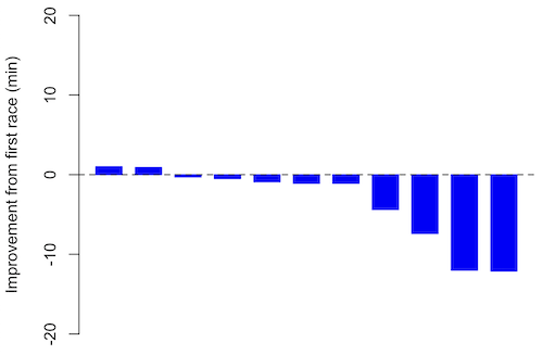
Figure 3. Simple waterfall plot of race improvement for Table 3 data. Dashed horizontal line at zero.
R code
Data wrangling: Create a new variable, eg, race21, by subtracting the first time from the second time. Multiply by -1 so that improvement (faster time in second race) is positive. Finally, apply descending sort so that improvement is on the left and increasingly poorer times are on the right.
df <- data.frame(
ID = rep(paste0("P", 1:11), each = 2),
Time = c(179.9,192.0,
129.9,130.8,
128.5,129.6,
179.4,179.7,
174.3,181.7,
177.2,176.2,
169.0,173.4,
174.1,175.2,
175.1,174.2,
163.9,175.9,
179.3,179.8)
)

# Convert to wide format
df_wide <- reshape(df, idvar = "ID", timevar = "ID",
direction = "wide")

# Extract first and second times manually
time_matrix <- matrix(df$Time, ncol = 2, byrow = TRUE)
colnames(time_matrix) <- c("Time1", "Time2")

# Calculate improvement (second - first)
base21 <- time_matrix[,2] - time_matrix[,1]

# Sort for waterfall display
base21 <- sort(base21, decreasing = TRUE)

# Waterfall plot
barplot(base21, col="blue", border="blue", space=0.5,
ylim=c(-20,20),
ylab="Improvement from first race (min)")
abline(h=0, lty=2)
Interpretation.
From the graph (Fig 3) we see that few of the racers improved their times the second time around — a few had decreased times.
Spaghetti plots.
Spaghetti plots, which display individual trajectories over time or multiple measurements, is a specialized line plot effective for visualizing the consistency of performance. The vertical thickness or spread of a single subject’s line across measurements indicates their level of repeatability. A “flat” line indicates high repeatability, while a volatile, zig-zagging line indicates low repeatability. Spaghetti plots are useful to visualize growth, decline, or stability over time for a single performance measure.
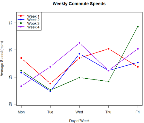
Figure 4. A spaghetti plot of average commute speeds from Table 2 data.
R code
# 1. Enter the data from Table 2.
commute <- data.frame(
Week = 1:4,
Monday = c(28.5, 25.8, 26.2, 23.3),
Tuesday = c(23.8, 22.4, 22.6, 26.9),
Wednesday = c(28.5, 29.3, 24.9, 31.3),
Thursday = c(30.2, 26.2, 24.2, 26.2),
Friday = c(26.9, 27.7, 34.3, 30.2)
)

head(commute)

# 2. Set the X-axis points
days <- 1:5
day_names <- c("Mon", "Tue", "Wed", "Thu", "Fri")

# 3. Create empty plot
# Find range of Y to ensure all data fits
ymin <- min(commute[, 2:6]) - 2
ymax <- max(commute[, 2:6]) + 2

plot(NA, xlim = c(1, 5), ylim = c(ymin, ymax),
xlab = "Day of Week", ylab = "Average Speed (mph)",
main = "Weekly Commute Speeds", xaxt = "n")

# Add X-axis labels
axis(1, at = 1:5, labels = day_names)

# 4. Add lines for each week (spaghetti)
colors <- c("red", "blue", "darkgreen", "purple")
for (i in 1:nrow(commute)) {
# Plot lines
lines(days, commute[i, 2:6], col = colors[i], lwd = 2, type = "b", pch = 19)
}

# 5. Add legend
legend("topleft", legend = paste("Week", 1:4), col = colors, lwd = 2, pch = 19)
Parallel coordinates plots.
Parallel coordinates plot allows each entity to be represented by a unique, continuous line traced across several vertical axes (each representing a different measurement or variable). High repeatability is indicated when a line remains roughly horizontal across all axes, while poor repeatability is visualized as lines that zig-zag or change direction between measurements.
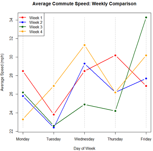
Figure 5. A parallel coordinates plot of average commute speeds from Table 2 data.
Both spaghetti plots and parallel coordinate plots can be used to visualize consistency of performance over multiple measures, but they differ significantly in their handling of data, scale, and context. Spaghetti plots are best for tracking within-subject variability over time, but quickly become a mess — like pasta tossed and sticking to a wall — when subject count increases. Parallel coordinate plots are a multivariate generalization — each line represents an individual’s profile across different tests, eg, accuracy, speed, VO2max.
R code.
# 1. Create the data frame
# see above

# 2. Extract only the numerical commute data for plotting
commute_data <- commute[, 2:6]

# 3. Setup the plot area
# Define range for y-axis
y_range <- range(commute_data)
# Define number of days (5)
num_days <- ncol(commute_data)

# Create empty plot
plot(NA, xlim = c(1, num_days), ylim = y_range,
xaxt = "n", xlab = "Day of Week", ylab = "Average Speed (mph)",
main = "Average Commute Speed: Weekly Comparison")

# Add x-axis labels
axis(1, at = 1:num_days, labels = colnames(commute_data))

# 4. Draw vertical lines for each day
for (i in 1:num_days) {
lines(c(i, i), y_range, col = "grey", lty = 2)
}

# 5. Add lines for each week (repeated measures)
colors <- c("red", "blue", "darkgreen", "orange")
for (i in 1:nrow(commute_data)) {
lines(1:num_days, commute_data[i, ], col = colors[i], lwd = 2, type = "b", pch = 19)
}

# 6. Add legend
legend("topleft", legend = paste("Week", commute$Week), col = colors, lwd = 2, pch = 19)
Heat map.
Heat map quickly identify patterns, such as an individual’s performance improving, degrading, or remaining stable over time. For example, uniform, solid colors across rows (individuals) or columns (time/trials) indicate high consistency, while varied colors indicate poor repeatability.
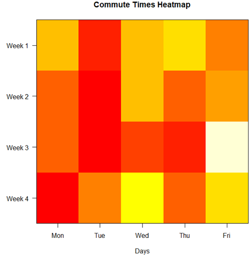
Figure 6. A heat map of the commute speeds data set.
R code.
# 1. Create the data
# Week is excluded from matrix to only include numerical commute times
commute_data <- matrix(c(
28.5, 23.8, 28.5, 30.2, 26.9,
25.8, 22.4, 29.3, 26.2, 27.7,
26.2, 22.6, 24.9, 24.2, 34.3,
23.3, 26.9, 31.3, 26.2, 30.2
), nrow = 4, byrow = TRUE)

# 2. Add row and column names
rownames(commute_data) <- c("Week 1", "Week 2", "Week 3", "Week 4")
colnames(commute_data) <- c("Mon", "Tue", "Wed", "Thu", "Fri")

# 3. Create the heatmap
# Use t() to transpose so weeks are rows and days are columns
# Use rev() on rows to have Week 1 at the top
image_data <- t(apply(commute_data, 2, rev))

# Set up the plotting area (margins for labels)
par(mar = c(5, 6, 4, 2))

# Plot the matrix
# Option 1
image(1:nrow(image_data), 1:ncol(image_data), image_data,
col = heat.colors(12),
axes = FALSE, xlab = "Days", ylab = "",
main = "Commute Times Heatmap")

# Add axes labels
axis(1, at = 1:5, labels = colnames(commute_data))
axis(2, at = 1:4, labels = rev(rownames(commute_data)), las = 1)
box()
Interpretation.
The graphs (Fig 4 – 6) show a lack of trends in consistency of drive speeds. The heat map suggests more consistency on Monday — low speeds (Fig 4 & Fig 5), but that’s a stretch.
An example for you to work, from our Measurement Day
If you recall, we had you calculate length and width measures on shells from samples of gastropod and bivalve species. In the table are repeated measures of shell length, by caliper in mm, for a sample of Conus shells (Fig 7 and Table 4).

Figure 7. Conus shells, image by M. Dohm.
Repeated measures of the same 12 Conus shells.
Table 4. Unstacked dataset of repeated length measures on 12 shells
| Sample | Measure1 | Measure2 | Measure3 |
|---|---|---|---|
| 1 | 45.74 | 46.44 | 46.79 |
| 2 | 48.79 | 49.41 | 49.67 |
| 3 | 52.79 | 53.45 | 53.36 |
| 4 | 52.74 | 53.14 | 53.14 |
| 5 | 53.25 | 53.45 | 53.15 |
| 6 | 53.25 | 53.64 | 53.65 |
| 7 | 31.18 | 31.59 | 31.44 |
| 8 | 40.73 | 41.03 | 41.11 |
| 9 | 43.18 | 43.23 | 43.2 |
| 10 | 47.1 | 47.64 | 47.64 |
| 11 | 49.53 | 50.32 | 50.24 |
| 12 | 53.96 | 54.5 | 54.56 |
Maximum length from from anterior end to apex with calipers. Repeated measures were conducted blind to shell id, sampling was random over three separate time periods.
Questions
- Consider data in Table 2, Table 3, and Table 4. True or False: The arithmetic mean is an appropriate measure of central tendency. Explain your answer.
- Enter the shell data into R; Best to copy and stack the data in your spreadsheet, then import into R or R Commander. Once imported, don’t forget to change Sample to character, otherwise R will treat Sample as ratio scale data type. Run your one-way ANOVA and calculate the intraclass correlation (ICC) for the dataset. Is the shell length measure repeatable?
- The marathon results in Table 2 are paired data, results of two races run by the same individuals. Make a profile plot for the data (see Ch10.3 for help).
- A profile plot is used to show paired data; for two or more repeat measures, use a line graph instead.
A. Produce a line graph for data in Table 4. The line graph is an option in R Commander (Rcmdr: Graphs Line graph…), and can be generated with the following simple R code:
lineplot(Sample, Measure1, Measure2, Measure3)
B. What trends, if any, do you see? Report your observations.
C. Make another line plot for data in Table 2. Report any trend and include your observations.
Quiz Chapter 12.3
Fixed effects, random effects, and agreement
Chapter 12 contents
- Introduction
- The need for ANOVA
- One way ANOVA
- Fixed effects, random effects, and agreement
- ANOVA from “sufficient statistics”
- Effect size for ANOVA
- ANOVA posthoc tests
- Many tests one model
- References and suggested readings
6.2 – Ratios and probabilities
Introduction
One common objective of a research project is comparison between quantities: one effective way to communicate a comparison is to construct a ratio. Ratios provide a standardized way to compare different data sets. The purpose of this page is introduce the wealth of types of ratios used for quantification of comparisons, from indexes to ratios.
Let’s review our definitions again. An event is some occurrence. As you know, a ratio is one number, the numerator, divided by another called the denominator. A proportion is a ratio where the numerator is a part of the whole. A rate is a ratio of the frequency of an event during a certain period of time. A rate may or may not be a proportion, and a ratio need not be a proportion, but proportions and rates are all kinds of ratios. If we combine ratios, proportions, and/or rates, we construct an index.
Ratios
Yes, data analysis can be complicated, but we start with this basic idea. Much of the statistics is based on frequency measures, eg, ratios, rates, proportions, indexes, and scales.
Ratios are the association between two numbers, one random variable divided by another. Ratios are used as descriptors and the numerator and denominator do not need to be of the same kind. Business and economics are full of ratios. For example, return on investment (ROI), eg, earnings equals net income divided by number of shares outstanding, the Price-Earnings, or P/E ratio, is the ratio of the price of a stock to the earnings per stock, as well as many others are used to summarize performance of a business, and to compare performance of one business against another.
Note 1: ROI also stands for region of interest — a sample in a data set identified by the analyst for a particular interest. Often refers to a specific area in an image.
Ratios are deceptively convenient way to standardize a variable for comparisons, ie, how many times one number contains another. For example, when estimating bird counts for different areas, or different birding effort (intensity, time searched), we may correct counts by accounting for area in which counts were made or the total time spent counting, for a per-unit ratio (Liermann et al 2004).
Practice: There were 1,326 day undergraduate students enrolled in 2014 at Chaminade University of Honolulu and the Sullivan Library added 8469 new items (ebooks, journals, etc,) to its collection during 2014. What is the ratio of new items per student?

Data collected from Chaminade University website at www.chaminade.edu on 3 July 2014.
Practice: For another example, what is ratio of annual institutional aid a student at Chaminade University may expect to receive compared to a student at Hawaii Pacific University?

Thus, in 2014, Chaminade offered more than twice the institutional aid to its students then does HPU (both institutions are private universities, data from retrieved on 3 July 2014 from www.cappex.com).
Relative change, Fold-change and orders of magnitude
It’s common practice to report on the amount of change between two quantities recorded over time. Relative change (often percentage) describes change relative to an initial value. Relative change in root length b
To make percent increase (decrease), simply multiple 100%.
(1) 
The ratio between two quantities, eg, to compare mRNA expression levels of genes from organisms exposed to different conditions, researchers may report fold-change. Fold change is often reported as log base 2 change.

Why log base 2? Symmetry and ease of reporting. A doubling becomes +1 and a halving becomes -1. Without log transformation, doubling is +2, but having is +0.5.
Relative change is useful for reporting percent changes, fold change for ratios, although if the change is small in amount, then relative change can be misleading, eg, value goes from five to ten, then the relative change is 100%, but effectively, a very small change in absolute units. Similarly, fold change becomes a large, but likely meaningless comparison, if the denominator is close to zero.
An example of calculation of fold change. Rates of the expression from cells exposed to heavy metal divided by expression under basal conditions. Gene expression under different treatments may be evaluated by calculating fold-change as the log base2 of the ratio of expression of a gene for one treatment divided by expression of same gene from control conditions. Copper is an essential trace element, but excess exposure to copper is known to damage human health, including chronic obstructive pulmonary disease. One proposed mechanism is that cell injury promotes an epithelial-to-mesenchymal shift. In a pilot study (N.I.H. INBRE P20RR016467), we investigated gene expression changes by quantitative real-time polymerase chain reaction (qPCR) in a rat lung Type II alveolar cell line exposed to copper sulfate compared to unexposed cells. Record cycle threshold values, CT, for each gene, where CT is number of cycles required for the fluorescent signal to exceed background levels; CT is inversely proportional to amount of cDNA (mRNA) in the sample. Genes investigated were ECAD, FOXC2, NCAD, SMAD, SNAI1, TWIST, and VIM, with ATCB as reference gene. ECAD expression is marker of epithelial cells, whereas FOXC2, NCAD, SNAI1, TWIST, and VIM expression marker of mesenchymal cells. After calculating  values, geometric means of normalized values of three replicates each are shown in Table 1.
Note 2: The  is a relative change quantification that relates the PCR signal of the normalized gene of interest (GOI) transcript in a treatment group to another sample, eg, an untreated control. is now a widely applied method to analyze the relative changes in gene expression from real-time quantitative PCR experiments (relevant papers on the analysis method, Livak and Schmittgen (2001) and Schmittgen and Livak (2008) have been cited more than 230K times, Pubmed 2026. See also Rao et al (2013).)
Log-transform, introduced in Ch03.2, was used because gene expression levels vary widely on the original scale and any log-transform will reduce the variability. log-base 2 specifically was used for fold-change in particular because it is easy to interpret (eg, see discussion in Bergemann and Wilson 2011 and Corliss et al 2024), and provides symmetry (all log-transforms provide this symmetry). For example, log(1/2, 2) returns -1, while log(2/1, 2) returns +1. Thus, base 2, we see a decrease by half or doubling of original scale is a fold change of  . In contrast,
log(1/2, 10) returns -0.301, while log(2/1, 10) returns +0.301 — which is perfectly accurate, but deceptive to interpret.
log-base 2 is commonly employed to calculate the number of bits — binary digits — for a given number of values. For example, 8 bits (0 – 7), then log2(8-1), and R returns 2.807355. Round, add 1, and the number of bits is3. Related R code, if want to calculate and print te binary representation of of a number, eg, 8, try
myBits <- intToBits(8)
paste(as.character(myBits),collapse="")
On a more casual note, log-base 2 is useful to calculate number of rounds for a single-elimination playoff tournament, eg, NCAA men’s and women’s basketball tournament or March Madness (NCAA). As of 2025, 60 teams are invited, plus the four winning teams from four play-in games, for a total of 64 teams. The number of rounds is log2(64) and R returns 6. These six are referred to as First Round, Second Round, Sweet Sixteen, Elite Eight, Final Four, and the Championship Game. The play-in games are referred to as the”First Four.” The function draw_bracket() of R package SwimmeR can be used to plot a simple playoff bracket.
Table 1. Mean and fold change of gene expression values from qPCR for several genes from a rat lung cell line.*
| Control | Copper-sulfate | Fold change | |
| ECAD | 34.6 | 35.7 | 0.6 |
| NCAD | 28.5 | 24.0 | 27.2 |
| SMAD | 29.5 | 25.0 | 28.2 |
| SNAI1 | 25.5 | 28.1 | 0.2 |
| FOXC2 | 27.6 | 27.0 | 1.9 |
| VIM | 23.1 | 16.4 | 134.4 |
| TWIST | 25.1 | 22.9 | 5.6 |
* INBRE funding, P20RR016467.
At face value, following four hour exposure to copper sulfate in media, some evidence that the epithelial cell line adopted gene expression profile of mesenchyme-like cells. However, weakness of fold-change is clear from Table 1: the quantity is sensitive to small values. ECAD expression in the cell line is low, thus high numbers of PCR cycles (mean = 36) and treated cells not much fewer (mean = 34.4).
Note 3: Calculation of is included. Geomean CT were
| Control | CuSO4 | |
| ACTB | 32.2 | 32.5 |
| NCAD | 28.5 | 24.0 |
For control cells, 
For treatment cells, 
and 
log2, 
table value differs by rounding
Orders of magnitude
In addition to fold change, order of magnitude is another common way to compare quantities. While fold change returns the multiplier between two numbers, order of magnitude generally refers to differences in multiples of ten, logarithmic.

Thus, a difference of one order of magnitude is the number multiplied by 101, three orders of magnitude is the number multiplied by 103, and so on. A change from 10 to 100 is a one order of magnitude increase; the same change, 10 to 100, is a ten-fold change. It’s a difference of scale. If a person’s salary increases by 3%, from $49K to $50,470, reporting this as an “order of magnitude” increase is nonsensical as a communication device (magnitude of change is just 0.01). By contrast, fold change for the same increase would be 1.03 — also indicative of a negligible increase, but a cleaner representation.
Rates
Rates are a class of ratios in which the denominator is some measure of time. For example, the four year graduation rate of some Hawaii universities are shown in Table 2.
Table 2. Percent students graduation with bachelor’s degrees within four years or six years (cohort 2014, data source NCES.ed.gov)
| School | Private/Public | Four-year, Percent graduation |
Six-year, Percent graduation |
| Chaminade University | Private (non-profit) | 43 | 58 |
| Hawaii Pacific University | Private (non-profit) | 31 | 46 |
| University of Hawaii – Hilo | Public | 15 | 38 |
| University of Hawaii – Manoa | Public | 35 | 62 |
| University of Hawaii – West Oahu | Public | 16 | 39 |
| University of Phoenix | Private (for profit) | 0 | 19 |
Examples of rates
Rates are common in biology. To name just a few
- Basal metabolic rate (BMR), often measured by indirect calorimetry, reported in units kiloJoules per hour.
- Birth rates and mortality (death) rates, components of population growth rate.
- Extinction rate, how often over a given time species go extinct.
- Growth rate, which may refer to growth of the individual (somatic growth rate), or increase of number of individuals in a population per unit time.
- Molecular clock hypothesis, rate of amino acid (protein) or nucleotide (DNA) substitution is approximately constant per year over evolutionary time.
- Mutation rate, frequency of new mutations in a DNA sequence of an organism over time.
- Photosynthetic rate, convert light energy into chemical energy.
- Phred quality score, error rates of incorrectly called nucleotide bases by the sequencer.
Proportions
Proportions are also ratios, but they are used to describe one part to the whole. For example, 902 women (self-reported) day undergraduate students enrolled in 2014 at Chaminade University in Honolulu, Hawaii.
Practice: Given that the total enrollment for Chaminade in 2014 was of 1,326, calculate the proportion of female students to the total student body.

More practice: A common statistic in agriculture is germination percentage, count the number of seeds that sprout over a period of time divided by total number of seeds planted multiplied by 100. Figure 1 shows an example of a germination trial for five tomato seeds. Seed in position 3 (left to right 1 – 5) failed to germinate, whereas the other four seeds display range of seedling growth. (A seed coat is observed next to plant 2.)

Figure 1. Example planting of five tomato seeds, day 5, on agar Petri dish (M. Dohm).
Observations conducted over 10 days. Germination defined as evidence of radicle by day 10. Data collected by student for biostatistics project. A random sample of results from three plates is presented in Table 3.
Table 3. Germination of tomato seeds on agar Petri dishes.
| Plate* | 1 | 2 | 3 | 4 | 5 |
| 18 | Yes | No | Yes | Yes | Yes |
| 13 | Yes | Yes | Yes | No | Yes |
| 20 | No | Yes | Yes | Yes | Yes |
* Random sample of three plates drawn from among 30 plates.
We calculate the percent germination for the 15 seeds planted as

Thus, for the sample of plates the germination percent was 80%, which, coincidently, is the same result if germination percent was calculated for the five seeds displayed in Figure 1.
Beginning in Chapter 7 – Probability, Risk Analysis, we introduce and use a number of proportions, for example incidence and prevalence are proportions, as is PPV — positive predictive value. Sensitivity and specificity are both proportions and also qualified as indexes.
Comparing proportions
In some cases you may wish to compare two proportions or two ratios. The hypothesis tested is the difference between the two ratios, and the test is if the confidence interval of the difference includes zero. If it does, then we would conclude there is no statistical difference between the two proportions. In R, use the prop.test function. For example, 63 women were on team sport rosters at Chaminade in 2014, a proportion of 59% of all student athletes (n = 106). Recall from the example above that women were 68% of all students at Chaminade University. Title IX compliance requires that a university “maintain policies, practices and programs that do not discriminate against anyone on the basis of gender” (NCAA, INCLUSION AND BELONGING Championing Women in Sports). In terms of athletic programs, then, universities are required to provide participation opportunities for women and men that are substantially proportionate to their respective rates of enrollment of full-time undergraduate students.
Consider Chaminade University: Is there a statistical difference between proportion of women athletes and their proportion of total enrollment? We introduce statistical inference in Chapter 8, but for now, this is a test of the null hypothesis that the difference between the two proportions is zero.
At the R prompt type (remember, anything after the # sign is a comment and ignored by R).
women = c(62,902)  #where 62 is the number of women athletes and 902 is the number of women students
students = c(106,1326)  #106 is the number of student athletes and 1326 is all students
prop.test(women,students)  #the default is a two-tailed test, ie, no group differences
And R returns
2-sample test for equality of proportions with continuity correction
 data: women out of students
X-squared = 3.6331, df = 1, p-value = 0.05664
alternative hypothesis: two.sided
95 percent confidence interval:
 -0.197532407 0.006861073
sample estimates:
 prop 1 prop 2
0.5849057 0.6802413
What is the conclusion of the test?
When you compare two groups, you’re asking whether the two groups are equal (the null hypothesis). Mathematically, that’s the same as saying the difference between the two groups is equal to zero.
First check the lower and upper limits of the confidence interval. A confidence interval is one way to report a range of plausible values for an estimate (see Ch 7.6 – Confidence intervals). It’s called a confidence interval because a probability is assigned to the range of values; a 95% confidence interval is interpreted as we’re 95% certain the true population value is somewhere between the reported limits. For our Chaminade University Title IX question, recall that we are asking whether the value of zero is included. The lower limit was -0.1975 and some change; the upper limit was 0.0068 and some change. Thus, zero is included and we would conclude that there was no statistical difference between the two proportions.
The second relevant output to look at is the p-value, or probability value. If the p-value is less than 5%, we typically reject the tested hypothesis. We will talk more about p-values and their relationship to inference testing in Chapter 8; for now, pay attention to the confidence interval (introduced in Chapter 3.4); if zero is included, then we conclude no substantial differences between the two proportions.
Indexes
Indexes are composite statistics that combine indicators. They condense complex diagnostic performance data into a single, universally understood numerical indicator.
Indexes are common in biology, and well-known business and economics indexes are reported on every day, eg, Dow Jones Industrial average combines stock prices from 30 companies listed on the New York Stock Exchange and the CPI, or Consumer Protection Index, constructed by the US Bureau of Labor Statistics from a “market basket of consumer goods and services, used by the government and other institutions to track inflation. The CPI itself is made up of numerous indexes to account for regional price differences and other factors.
Some indexes presented in this book include
- Grade point average
- Body Mass Index (BMI)
- Comet assay indexes (tail intensity, tail length, tail moment) are used to assess DNA damage among organisms exposed to environmental contaminants (eg, Mincarelli et al., 2019).
- Encephalization index, ratio of brain to body weight among species. Used to compare cognitive abilities.
- Sensitivity, specificity, NNT — number needed to treat, odds-ratio and RRR and related. See Chapter 7.1 – Probability, Risk Analysis.
- Species diversity indexes, measures of species richness and abundance. See Chapter 20.8.
Scales
Agreement scales for surveys, eg, Likert scale or sliding scale (Sullivan and Artino 2013). For example, after learning about Theranos, students were asked:
How serious is this violation in your opinion?
| Not serious
0 |
Slightly serious
0 |
Moderately serious
2 |
Serious
4 |
Very serious
19 |
a 5-point scale.
Although an intuitive measure, how fast can an individual run, challenging to determine whether individual’s performance is at physiological maximum. Particularly for measures of performance capacity that involves behavior (motivation), may apply a race quality scale (eg., binary scale “good” or “bad” Husak et al 2006).
These examples reflect ordinal scales. Many of the nonparametric tests discussed in Chapter 15 are suitable for analysis of scales.
Limitations of ratios
Although the indexes may be easy to communicate, statistically, indexes have many drawbacks. Chief among these, variation in ratios may be due to change in numerator or denominator. Ratios and any index calculated by combining ratios seem simple enough, but have complicated statistical properties. Over the years, several authors have made critical suggestions for use of ratios and indexes. Some key references are Packard and Boardman (1988), Jasienski and Oikos (1999), Nee et al (2005), and Karp et al (2012). For example, ratios, computing trait value by body weight, are often used to compare some trait among individuals or species that differ in body size. However, this normalization attempt only removes the covariation between size and the trait if there is a 1:1 relationship between size and the trait. More typically, relationship between the trait and body size is allometric, ie, the slope is not equal to one. Thus, ratio will over-correct for large size and under-correct for small size. The proper solution is to conduct the comparison as part of an analysis of covariance (ANCOVA, see Chapter 17.6).
Example
Which is the safer mode of travel: car or airplane?
The following discussion covers travel safety in the United States of America for a typical year, 2000*.
Note 4: *The following discussion excludes the 241 airline passenger deaths associated to the terrorist attacks of September 11 2001 in the USA; the NTSB also “…exclude(s illegal acts) for the purpose of accident rate computation. It also does not include considerations of 2020-2021 and effects of the COVID-19 pandemic on numbers of flights. The purpose of this discussion is not to convince you about the safety of modes of travel. Moreover, the following analysis is not necessarily the proper way to frame or analyze risk, but, rather, the purpose of this discussion is to highlight the impact of assumptions on estimating risk.
Between 2000 and 2023, there were 779 deaths associated with accidents of major air carriers in the USA. Year 2009 was the last multiple-casualty crash of a major U.S. carrier (Colgan Air Flight 3407); between 2010 and 2021, two fatal accidents, two fatalities were reported.
We’ve all heard the claim that it’s much safer to fly with a major airline than it is to travel by car (eg, Flying is getting scary. But is it still safe? CNN June 20, 2024). There are a variety of arguments, but one statistical argument goes as follows. In 2000 in the United States, 638,902,993 persons traveled by major air carrier, whereas there were 190,625,023 licensed drivers. In 2000, 92 persons died in air travel (again, major carriers only), whereas 37,526 persons died in vehicle crashes (includes drivers and passengers). Thus, the risk of dying in air travel is given as the proportion  , or 1.44e-07 (0.000014%), whereas the comparable proportion for death by motor vehicle is
 , or 1.97e-04 (0.0197%).
In other words, we can expect one death (actually 1.4) for every ten million airline passengers, but 20 deaths (actually 19.7) for every one hundred thousand licensed drivers. Thus, flying is a thousand times safer than driving (actual result 1,367 times; divide the rate of motor vehicle-caused deaths for licensed drivers by the rate for airlines). Proportions are hard to compare sometimes, especially when the per capita numbers differ (ten million vs. 100,000 in this case).
We can put the numbers onto a probability tree and get a sense of what we are looking at (Fig 2).
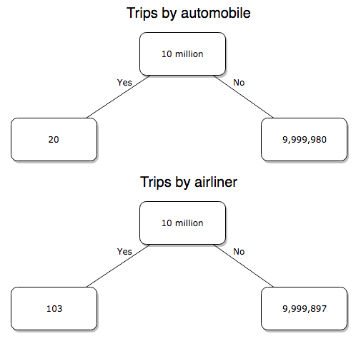
Figure 2. A probability tree to help visualize comparison of deaths (“yes”) by car travel and by airline travel in the United States for the year 2000.
Comparing rates and proportions
Without going into the details, we will do so in Chapter 9 Inferences on Categorical Data, comparing two rates is a chi-square, χ2, contingency table type of problem. More specifically, however, it is a binomial problem (Chapter 3.1, Chapter 6.5); there are two outcomes, death or no death, and we can describe how likely the event is to occur as a proportion. Because the numbers are large, we can use rely on the normal distribution for comparing the two proportions. We’ll explain this more in the next chapters, but for now it may be enough to present the equation for the comparison of two proportions under the assumption of normality, proportion z test.
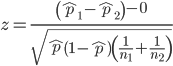
and the null hypothesis (see Chapter 8) tested as that the two proportions are equal. This may be written as
H0 : p1-p2=0
We can assign statistical significance to the differences in events for the two modes of travel under this set of assumptions. Rcmdr has a nice menu-driven system for comparing proportions, but for now I will simply list the R commands.
At the R prompt type each line then submit the command.
total = 100000000
prop.test(c(19700,14),c(total,total)))
And the R output
prop.test(c(19700,14),c(total,total))

    2-sample test for equality of proportions with continuity
    correction

data:  c(19700, 14) out of c(total, total)
X-squared = 19658, df = 1, p-value < 2.2e-16
alternative hypothesis: two.sided
95 percent confidence interval:
 0.0001940984 0.0001996216
sample estimates:
  prop 1   prop 2
1.97e-04 1.40e-07
There’s a bit to unpack here. R is consistent; when it reports results of a statistical test, it typically returns the value of the test statistic (χ2 = 19658), the degrees of freedom for the test (df = 1), and the p-value (< 2.2e-16).
prop.test() were calculated by the Wilson Score method not the Wald method. While both are parametric tests and therefore sensitive to departures from normality (see Chapter 13.3), formulation of Wilson score method makes fewer assumptions (involving approximations of the population proportions) and therefore is considered more accurate.By convention in statistics, if a p-value, where “p” stands for probability, is less than 5%, we would say that our results are statistically significant from the null hypothesis. Looks pretty convincing to me, the difference of 19,700 deaths compared to 14 deaths is clearly different by any criterion and by the results of the statistical test, the p-value is several orders of magnitude smaller than 5%.
Safer to fly. By far, not even close. And similar conclusions would be reached if we compare different years, or averages over many years, or if we used a different way to express the amount of travel (eg, miles/year) by these modes of transportation.
Are you convinced, really? Is it safer to fly?
Let’s try a little statistical reasoning — what assumptions did I make to do these calculations? We recognize immediately that many more people travel by car: that there are way more cars being driven then there are airline planes being flown. The question then is, have we properly adjusted for this difference? Here are a few considerations. My source for the numbers is the NTS 2001 book published by the U.S. Department of Transportation (U.S. Department of Transportation). We are conducting a risk analysis, and the first step is to make sure that we are comparing “apples with apples.” Here are two alternative solutions that at least compare, “Red Delicious” apples with “Macintosh” apples.
Option 1. There are many, many more licensed drivers than there are licensed commercial airline pilots. The standard comparison offered in the background above compared deaths per licensed car driver, but a different metric for air travel, the rate per passenger. This isn’t as bad of a comparison as it may seem — after all, the majority of deaths in car accidents are of the driver themselves. But it isn’t that hard to make the direct comparison — just find out how many commercial pilots there are — a direct comparison with licensed car drivers (stated above as 190,625,023). From the FAA we see that in 2009 there were 125,738 persons with commercial certificates. Since there are only 20 major airline carriers in the United States now (a few more were active in 2000, but we’ll put this aside), the number of licenses is an over estimate of the actual number we want — how many pilots of commercial airlines — but lets use this number for starters — after all, just because a person has a drivers license doesn’t mean they drive or ride in a car.
Number of deaths/yr: Let’s use 2000 data, a typical year prior to 9/11 (and excluding the Covid-19 pandemic). Airlines: 92 deaths; motor vehicles (includes passenger cars, trucks, etc, but not motorcycles): 37,526 deaths (drivers = 25,567; passengers = 10,695; 86 others).
Which mode of travel is riskier? I get a rate a rate of 7.3 X 10⁻⁴ deaths per commercial pilot, or
92125738
compared to a rate for car drivers of 1.97 X 10⁻⁴ deaths.
To summarize what we have so far, I get a result that suggests car travel is almost four times safer
7.3 x 10-41.97 x 10-4→7.31.97 = 3.7
then traveling by commercial airliner. In whole numbers, these results translate to seven deaths for every 10,000 commercial pilots compared to two deaths for every 10,000 licensed car drivers (Fig 3).
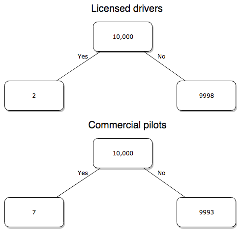
Figure 3. Comparing totals of deaths adjusted by numbers of licensed drivers and by licensed commercial airline pilots in the United States.
R work follows. Enter and submit each command on a separate line in the script window
total = 10000
prop.test(c(2,7),c(total,total))
And the R output
prop.test(c(2,7),c(total,total))

    2-sample test for equality of proportions with continuity
    correction

data:  c(2, 7) out of c(total, total)
X-squared = 1.7786, df = 1, p-value = 0.1823
alternative hypothesis: two.sided
95 percent confidence interval:
 -0.001187816  0.000187816
sample estimates:
prop 1 prop 2
 2e-04  7e-04
What’s happened? The p-value (0.1823) is not less than 5% and so we would conclude under this scenario that there is no difference between the proportions of deaths between the two modes of travel. Let’s keep going.
Option 2. There are many, many more cars on the road then there are airplanes flying commercial passengers. The standard comparison offered in the background information above identified death rates per individual driver, but used a different metric for airline travelers (number of deaths per passenger), which confuses individuals with travelers: what we need is the number of individuals that traveled by airliner, not the total number of passengers (which is many times higher, because of repeat flyers). How can we make a fair comparison for the two modes of travel? Most people never fly whereas most people drive (or ride in a car) frequently in the United States. To me, risk of travel might be better expressed in terms of a per trip rate. I want to know, what are my chances of dying each time I get into my car versus each time I fly on a commercial jet in the United States?
Number of trips/yr. For airlines, I use the number of departures (2000 = 8,951,773). But for cars, we need to decide how to get a similar number. It’s not available directly from the DOT (and would be difficult to get — studies with randomly selected drivers can yield as many as 5 trips per day for licensed drivers). I took the number of licensed drivers and bound the problem — at the low end, let’s say that only 2 trips per week (eg, 50 weeks) are taken by licensed drivers (100 trips); at the upper end, let’s take 2 trips per day per week, or 500 trips/year. Thus, at the low end, we have 1.91 X10¹⁰ trips per year; at the upper end, 9.53 X 10¹⁰ trips per year.
Which mode of travel is riskier? Using the number of deaths/yr listed above in Option 1, I get a rate of 1.03 X 10⁻⁵ deaths/trip for air carriers
928.95 x 10⁶
compared to a rate of 1.97 X 10⁻⁶ deaths/trip for cars (lower bound) or 3.9 X 10⁻⁷ deaths/trip for cars (upper bound). Here’s what the numbers look for in a tree (taking the lower number of trips per year for cars, Fig 4).
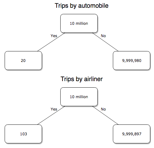
Figure 4. Comparing totals of deaths adjusted by numbers of car trips and by numbers of airline trips in the United States.
R work follow
total = 10000000
prop.test(c(20,103),c(total,total))
And the R output
prop.test(c(20,103),c(total,total))

    2-sample test for equality of proportions with continuity
    correction

data:  c(20, 103) out of c(total, total)
X-squared = 54.667, df = 1, p-value = 1.428e-13
alternative hypothesis: two.sided
95 percent confidence interval:
 -1.057370e-05 -6.026305e-06
sample estimates:
  prop 1   prop 2
2.00e-06 1.03e-05
Now we have another really small p-value (1.428e-13), which suggests a statistically significant difference between the modes of air travel, but the difference in deaths is switched. I now have a result that suggests car travel is much safer than traveling with a commercial airliner! These calculations suggest that you are as much as 26 (upper bounds, five times for lower bounds) times more likely to die from a plane crash then you are behind the wheel. In whole numbers, these results indicate one death for every 100,000 airline flights compared to 1 death for every 500,000 (lower estimate) or 2,500,000 car trips!
Do I have it right and the standard answer is wrong? As Lee Corso used to say on ESPN’s College GameDay program, “Not so fast, my friend!” (Wikipedia). Mark Twain was right to hold the skeptic’s view. Begin by listing the assumptions and by checking the logic of the comparisons (there are still holes in my logic!!). For one, if I am considering my risk of dying by mode of travel, it is far more likely that I will be in a car accident than I will an airline accident, simply because I don’t travel by airline that much. When we consider lifetime risk, we can see why the assertion that it is “safer to fly than drive” is true — we’re far more likely to belong to one of the reference populations involving automobiles (eg, those who drive frequently, for many years) than we are to be among the frequent flyers reference populations.
Questions
1. Review and provide your own examples for
- index
- rate
- ratio
- proportion
3. Like travel safety, we are often confronted by risk comparisons like the following: Which animal is more deadly to humans, dogs or sharks? Between the two, which lead to more hospitalizations in the United States? Work through your assumptions and use results from the International Shark Attack file.
- If a person lives in Nebraska, and never visits the ocean, how does a “shark attack” risk analysis apply? Is it a fair comparison to make between dog attacks and shark attacks? Why or why not.
4. Go to cappex.com/colleges and update institutional (gift) aid offered by Chaminade and HPU. Compare to University of Hawaii-Manoa.
5. Calculate percent increase for
- Annual atmospheric CO2 1980 and 2024.
Quiz Chapter 6.2
Ratios and probabilities
Chapter 6 content
- Introduction
- Some preliminaries
- Ratios and probabilities
- Combinations and permutations
- Types of probability
- Discrete probability distributions
- Continuous distributions
- Normal distribution and the normal deviate (Z)
- Moments
- Chi-square distribution
- t distribution
- F distribution
- References and suggested readings
10 – Inferences, Quantitative: Two Sample tests
Testing differences in averages: From one group to two
A one sample parametric test compares the mean against a population value. The population value may come literally from census information, or, more likely, it comes from some applicable theory. The one sample t-test was presented along with how to calculate the confidence interval in the previous chapter.
In this chapter, we also extend to consider two samples, tests about hypotheses for two groups. The two groups may consist of observations on different subjects, and thus the two groups are independent of each other — an independent sample t-test may be used to test null hypothesis. This is called a crossed design or between-subjects design –where each group has its own unique set of observations, and no relationship exists between the observations in the two groups. We discuss crossed experimental designs in Chapter 14.1.
A common experimental design is to measure individuals two or more times, eg, observations like body mass index, BMI, recorded on individuals at the start of an exercise program, and again on the same individuals some time after a treatment — a repeated measures design. In this case, the measures are paired and are, thus, not independent, and a paired-sample t-test would be advised. If the repeated measures occur at different times, then the design is also longitudinal design or within-subjects design. Paired data are examples of nested design — the data points are clustered within individual units. We discuss nested experimental designs in Chapter 14.5.
Two sample parametric tests are used to answer questions about the mean where the data are collected from two random samples of independent observations, each from an underlying normal distribution. The samples may be independent or paired, in which different hypotheses are tested.
Suggested homework
Quizzes in this chapter
A total of 27 questions among the several subchapters, a mix of true or false and multiple choice question format.
Chapter 10 contents
- Introduction
- Compare two independent sample means
- Digging deeper into t-test Plus the Welch test
- Paired t-test
- References and suggested reading
8.6 – Confidence limits for the estimate of population mean
Introduction
In Chapter 3.4 and Chapter 8.3, we introduced the concept of providing a confidence interval for estimates. We gave a calculation for an approximate confidence interval for proportions and for the Number Needed to Treat (Chapter 7.3). Even an approximate confidence interval gives the reader a range of possible values of a population parameter from a sample of observations.
In this chapter we review and expand how to calculate the confidence interval for a sample mean,  . Because is derived from a sample of observations, we use the t-distribution to calculate the confidence interval. Note that if the population was known (population standard deviation), then you would use normal distribution. This was the basis for our recommendation to adjust your very approximate estimate of a confidence interval for an estimate by replacing the “2” with “1.96” when you multiply the standard error of the estimate (SE) in the equation estimate
 . As you can imagine, the approximation works for large sample size, but is less useful as sample size decreases.
Consider ; it is a point estimate of  , the population mean (a parameter). But our estimate of is but one of an infinite number of possible estimates. The confidence interval, however, gives us a way to communicate how reliable our estimate is for the population parameter. A 95% confidence interval, for example, tells the reader that we are willing to say (95% confident) the true value of the parameter is between these two numbers (a lower limit and an upper limit). The point estimate (the sample mean) will of course be included between the two limits.
Instead of 95% confidence, we could calculate intervals for 99%. Since 99% is greater than 95%, we would communicate our certainty of our estimate.
Note 1: Again, the caveats about p-value extend to confidence intervals. See Chapter 8.2.
Question 1: For 99% confidence interval, the lower limit would be smaller than the lower limit for a 95% confidence interval.
- True

- False
When we set the Type I error rate,  (alpha) = 0.05 (5%), that means that 5% of all possible sample means from a population with mean, , will result in t values that are larger than
 OR smaller than
 .
Why the t-distribution?
We use the t-test because, technically, we have a limited sample size and the t-distribution is more accurate than the normal distribution for small samples. Note that as sample size increases, the t-distribution is not distinguishable from the normal distribution and we could use  (Fig 1).
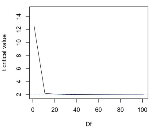
Figure 1. Critical values at Type I rate of 5% of t-distribution  . Blue dashed line is z = 1.96.
Here’s the equation for calculating the confidence interval based on the t-distribution. These set the limits around our estimate of the sample mean. Together, they’re called the 95% confidence interval,  .

Here’s a simplified version of the same thing, but generalized to any Type I level…
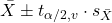
This statistic allows us to say that we are 95% confident that the interval includes the true value for . For this confidence interval you need to identify the critical t value at 5%. Thus, you need to know the degrees of freedom for this problem, which is simply  , the sample size minus one.
It is straightforward to calculate these by hand, but…
Set the Type I error rate, calculate the degrees of freedom (df):
 samples for one sample test
- pairs of samples for paired test
 samples for two independent sample test
and lookup the critical value from the t table (or from the t distribution in R). Of course, it is easier to use R.
In R, for the one tail critical value with seven degrees of freedom, type at the R prompt
qt(c(0.05), df=7, lower.tail=FALSE)
[1] 1.894579
For the two-tail critical value
qt(c(0.025), df=7, lower.tail=FALSE)
[1] 2.364624
Or, if you prefer to use R Commander, then follow the menu prompts to bring up the t quantiles function (Fig 2 and Fig 3).
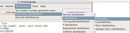
Figure 2. Drop down menu to get t-distribution.
Note 2: Quantiles divide probability distribution into equal parts or intervals. Quartiles have four groups, deciles have ten groups, and percentiles have 100 groups.

Figure 3. Menu for t quantiles, with values entered for the two-tail example.
You should confirm that what R calculates agrees with the critical values tabulated in the Table of Critical values for the t distribution provided in the Appendix.
A worked example
Let’s revisit our lizard example from last time (see Chapter 8.5). Prior to conducting any inference test, we decide acceptable Type I error rates (cf justify alpha discussion in Ch8.1); For this example, we set Type I error rate to be 1% for a 99% confidence interval.
The Rcmdr output was
t.test(lizz$bm, alternative='two.sided', mu=5, conf.level=.99)
data: lizz$bm
t = -1.5079, df = 7, p-value = 0.1753
alternative hypothesis: true mean is not equal to 5
99 percent confidence interval:
1.984737 6.199263
sample estimates:
mean of x
4.092
Sort through the output and identify what you need to know.
Question 1: What was the sample mean?
- 5
- -1.5079
- 7
- 0.1753
- 1.984737
- 6.199263
- 4.092
Question 2: What was the most likely population mean?
- 5
- Answer
- -1.5079
- 7
- 0.1753
- 1.984737
- 6.199263
- 4.092
Question 3: This was a “one-tailed” test of the null hypothesis?
- True
- False
The output states “alternative hypothesis: true mean is not equal to 5” — so it was a two-tailed test.
Question 4: What was the lower limit of the confidence interval?
- 5
- -1.5079
- 7
- 0.1753
- 1.984737
- 6.199263
- 4.092
The 99% confidence interval,  , is
 , which means we are 99% certain that the population mean is between
 (lower limit) and
 (upper limit). In Chapter 8.5 we calculated the , is
 .
Confidence intervals by nonparametric bootstrap sampling.
Bootstrapping is a general approach to estimation or statistical inference that utilizes random sampling with replacement (Kulesa et al. 2015). In classic frequentist approach, a sample is drawn at random from the population and assumptions about the population distribution are made in order to conduct statistical inference. By resampling with replacement from the sample many times, the bootstrap samples can be viewed as if we drew from the population many times without invoking a theoretical distribution. A clear advantage of the bootstrap is that it allows estimation of confidence intervals without assuming a particular theoretical distribution and thus avoids the burden of repeating the experiment. Which method to prefer? For cases where assumption of a particular distribution is unwarranted (eg, what is the appropriate distribution when we compare medians among samples?), bootstrap may be preferred (and for small data sets, percentile bootstrap may be better). We cover bootstrap sampling of confidence intervals in Chapter 19.2 Bootstrap sampling.
Conclusions
The take home message is simple.
- All estimates should — must? — be accompanied by a Confidence Interval
- The more confident we wish to be, the wider the confidence interval will be
Note that the confidence interval concept combines DESCRIPTION (the population mean is between these limits) and INFERENCE (and we are 95% certain about the values of these limits). It is good statistical practice to include estimates of confidence intervals for any estimate you share with readers. Any statistic that can be estimated should be accompanied by a confidence interval and, as you can imagine, formulas are available to do just this. For example, earlier this semester we calculated NNT.
Questions
- To gain practice with calculations of confidence intervals, calculate the approximate confidence interval, the 95% and the 99% confidence intervals based on the t distribution, for each of the following.
-
- = 13,
 = 1.3,
 = 10
- = 13, = 1.3, = 30
- = 13, = 2.6, = 10
- = 13, = 2.6, = 30
Quiz Chapter 8.6
Confidence limits for the estimate of population mean
Chapter 8 contents
- Introduction
- The null and alternative hypotheses
- The controversy over proper hypothesis testing
- Sampling distribution and hypothesis testing
- Tails of a test
- One sample t-test
- Confidence limits for the estimate of population mean
- References and suggested readings
8.3 – Sampling distribution and hypothesis testing
Introduction
Understanding the relationship between sampling distributions, probability distributions, and hypothesis testing is the crucial concept in the NHST — Null Hypothesis Significance Testing — approach to inferential statistics. is crucial, and many introductory text books are excellent here. I will add some here to their discussion, perhaps with a different approach, but the important points to take from the lecture and text are as follows.
Our motivation in conducting research often culminates in the ability (or inability) to make claims like:
- “Total cholesterol greater than 185 mg/dl increases risk of coronary artery disease.”
- “Average height of US men aged 20 is 70 inches (1.78 m).”
- “Species of amphibians are disappearing at unprecedented rates.”
Lurking beneath these statements of “fact” for populations (just what IS the population for #1, for #2, and for #3?) is the understanding that not ALL members of the population were recorded.
How do we go from our sample to the population we are interested in? Put another way — How good is our sample? We’ve talked about how “biostatistics” can be generalized as sets of procedures you use to make inferences about what’s happening in populations. These procedures include:
- Have an interesting question
- Experimental design (Observational study? Experimental study?)
- Sampling from populations (Random? Haphazard?)
- Hypotheses: HO and HA
- Estimate parameters (characterize the population)
- Tests of hypotheses (inferences)
We have control of each of these — we choose what to study, we design experiments to test our hypotheses…We have already introduced these topics (Chapters 6 – 8).
We also obtain estimates of parameters, and inferential statistics applies to how we report our descriptive statistics (Chapter 3). Estimates of parameters like the sample mean and sample standard deviation can be assessed for accuracy and precision (eg, confidence intervals).
Sampling distribution
Imagine drawing a sample of 30 from a population, calculating the sample mean for a variable (eg, systolic blood pressure), then calculating a second sample mean after drawing a new sample of 30 from the same population. Repeat, accumulating one estimate of the mean, over and over again. What will be the shape of this distribution of sample means? The Central Limit Theorem states that the shape will be a normal distribution, regardless of whether or not the population distribution was normal, as long as the sample size is large (ie, Law of Large Numbers). We alluded to this concept when we introduced discrete and continuous distributions (Chapter 6).
It’s this result from theoretical statistics that allows us to calculate the probability of an event from a sample without actually carrying out repeated sampling or measuring the entire population.
A worked example
To demonstrate the CLT we want R to help us generate many samples from a particular distribution and calculate the same statistic on each sample. We could make a for loop, but the replicate() function provides a simpler framework. We’ll sample from the chi-square distribution. You should extend this example to other distributions on your own, see Question 5 below.
Note 1: This example is much simpler to enter and run code in the script window, modifying code directly as needed. If you wish to try to run this through Rcmdr, you’ll need to take a number of steps, and likely need to modify the code and rerun anyway. Some of the steps in would be Rcmdr: Distributions → Continuous distributions → Chi-squared distribution → Sample from chi-square distribution…, then running Numerical summaries and saving the output to an object (eg, out), extracting the values from the object (eg, out$Table, confirm by running command str(out)— str() is an R utility to display the structure of an object), then testing the object for normality Rcmdr: Statistics → Test of normality, select Shapiro-Wilk, etc.. In other words, sometimes a GUI is a good idea, but in many cases, work with the script!
Generate x replicate samples (eg, x = 10, 100, 1000, one million) of 30 each from chi-square distribution with one degree of freedom, test the distribution against null hypothesis (assume normal distributed, eg, Shapiro-Wilk test, see Chapter 13.3), then make a histogram (Chapter 4.2), like Figure 1 or Figure 2.
x.10 <- replicate(10, {
my.mean <- rchisq(30, 1)
mean(my.mean)
})

normalityTest(~x.10, test="shapiro.test")
hist(x.10, col="orange")
Result from R
Shapiro-Wilk normality test

data: x.10
W = 0.87016, p-value = 0.1004
Figure 1. means of ten replicate samples drawn at random from chi-square distribution, df = 1.
Modify the code to draw 100 samples, we get Fig 2.
Figure 2. means of 100 replicate samples drawn at random from chi-square distribution, df = 1. Results from Shapiro-Wilks test: W = 0.97426, p-value = 0.04721.
And finally, modify the code to draw one million samples, we get Figure 3.
Figure 3. means of one million replicate samples drawn at random from chi-square distribution, df = 1. Normality test will fail to run, sample size of 5000 limit.
How to apply sampling distribution to hypothesis testing
First, a reminder of some definitions.
Estimate = we will always (almost) concern ourselves with how good our sample mean (such values are called estimates) is relative to the population mean, the thing we really want, but can only hope to get an estimate of.
Accuracy = how close to the true value is our measure?
Precision = how repeatable is our measure?
How can we tell if we have a good estimate? We want an estimate with an evaluation for accuracy and for precision. The sampling error provides an assessment of precision, whereas the confidence interval provides a statement of accuracy. We need an estimate of the sampling error for the statistic,
Sample standard error of the mean
We introduced sample error of the mean in section 3.4 of Chapter 3. Everything we measure can have a corresponding statement about how accurate (sampling error) is our estimate! First, we begin by asking, “how accurate is the mean that we estimate from a sample of a population?” How do we answer this? We could prove it in the mathematical sense of proof (and people have and do) OR we can use the computer to help. We’ll try this approach in a minute.
What we will show relates to the standard error of the population mean (SEM) or

, whose equation is shown below.

or equivalently, from the standard deviation we have
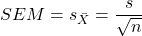
Note that the SEM takes the variance and divides through by the sample size. In general, then, the larger the sample size, the smaller the “error” around the mean. As we work through the different statistical tests, t-tests, analysis of variance, and related, you will notice that the test statistic is calculated as a ratio between a difference or comparison divided by some form of an error measurement. This is to remind you that “everything is variable.”
A note on standard deviation (SD) and standard error of the mean (SEM): SD estimates the variability of a sample of Xi‘s whereas SEM estimates the variability of a sample of means.
Let’s return to our thought problem and see how to demonstrate a solution. First, what is the population? Second, can we get the true population mean?
One way, a direct (but impossible?) approach would be to measure it — get all of the individuals in a population and measure them, then calculate the population mean. Then, we could compare our original sample mean against the true mean and see how close it was. This can be accomplished in some limited cases. For example, the USA conducts a census of her population every ten years, a procedure which costs billions of dollars. We can then compare samples from the different states or counties to the USA mean. And these statistics are indeed available via the census.gov website. But even the census uses sampling — individuals are randomly selected to answer more questions and from this sample trends in the population are inferred.
So, sampling from populations is the way to go for most questions we will encounter. The procedures we will use to show how a sample mean relates to the population mean are general and may be used to show how any estimate of a variable (sample mean and sample standard deviation, etc.), relates to properties of a parameter. We’ll get to the other issues, but for now, think about sample size.
Sampling from populations is necessary and inevitable, and, to a certain extent, under your control. But how many individuals do we need? The quick answer is for me to direct your attention to the equation for the SEM. Can you see in that ratio the secret to obtaining more precise estimates? There are many ways to approach this question, but let’s use the tools from last time, those based on properties of a normal distribution.
If we can view the sampling as having come from a population at least approximately normally distributed for our variable, then we can now examine empirically the effect of different sample sizes on the estimate of the mean.
A hint: variability is important!
From one population we obtain two samples, A and B. Sample sizes are
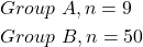
Assume for now that we know the true mean (μ) and standard deviation (σ) for the population. Note. This is one of the points of why we use computer simulation so much to teach statistics — it allows us to specify what the truth is, then see how our statistical tools work or how our assumptions affect our statistically based conclusions.
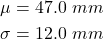
Confidence intervals
Reliability is another word for precision. We define a confidence interval as a statistic to report the reliability of our estimated statistic. We introduced confidence interval in Chapter 3.4. At least in principle, confidence intervals can be calculated for all statistics (mean, variance, etc.,) and for all data types. Confidence intervals define a lower limit, L, and an upper limit, U, and that you are making a statement that you are “95% certain that the true value (parameter value) is between these two limits.
We previously reported how to calculate an approximate confidence intervals for proportions and for NNT; simply multiple standard error estimate by 2. Here we introduce an improved approximate calculation of the 95% confidence interval for the sample mean

where Z is something you would look up from the table of the normal distribution. For a 95% confidence interval, 100% – 95% = 5% and divide 5% by two: the lower limit corresponds to 2.5% and the upper limit corresponds to 2.5% on our normal distribution. We look up the table and we find that Z for 0.025 is 1.96 and that is the value we would plug into our equation above. For large sample sizes, you can get a pretty decent estimate of the confidence interval by replacing 1.96 with “2.”
Questions
1. What is the probability of having a sample mean greater than 50 (mean > 50) for a sample of n = 9 ?
We’ll use a slight modification of the Z-score equation we introduced in Chapter 6.6 — the modification here is that previously we referred to the distribution of Xi‘s and how likely a particular observation would be. Instead, we can use the Z score with the standard normal distribution (aka Z-distribution), approach to solving how likely an estimated sample mean is given the population parameters μ and σ. Recall the Z score

We have everything we need except the SEM, which we can calculate by dividing the standard deviation by squared root of sample size.
For

, σ = 12.0 (given above), and μ = 47, n = 9, plug in the values:
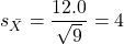
Therefore, after applying the equation for Z score,  . This corresponds to how far away from the standard mean of zero.
Look up from the table of normal distribution. The answer is  , which corresponds to that
 is EQUAL to or GREATER than 0.75, which is what we wanted. Translated, this implies that, given the level of variability in the sample, 22.66% of your sample means would be greater than 50! We write:
 .
Some care needs to be taken when reading these tables — make sure you understand how the direction (less than, greater than) away from the mean is tabulated.
2. Instead of greater, how would you get the probability less than 50?
Total area under the curve is 1 (100%), so subtract  .
I recommend that you do these by hand first, then check your answers. You’ll need to be able to do this for exams.
Here’s how to use Rcmdr to do these kind of problems.
Rcmdr: Distributions → Continuous distributions → Normal distribution → Normal probabilities …
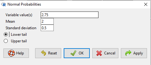
Figure 5. Screenshot Rcmdr menu to get normal probability.
Here’s the answer from Rcmdr
pnorm(c(50), mean=47, sd=12, lower.tail=TRUE)

[1] 0.5987063
3. Now, try a larger sample size. For  , what is the probability of having a sample mean greater than 50 (
 )?
, μ = 47, σ = 12, n = 50 and

Therefore, after applying the equation for Z score,  . Look up (Normal table, subtract answer from 1) and we get
 .
Or 3.84% of your sample means would be greater than 50! We write:  .
Said another way: If you have a sample size of 50 () and you obtain a mean greater than 50 then there is only a 3.84% chance that the TRUE MEAN IS 47.
4. What happens if the variability is smaller? Chance σ from 12 to 6 then repeat questions 1 and 4.
5. Repeat the demonstration of Central Limit Theorem and Law of Large Numbers for discrete distributions
- binomial distribution. Replace
rchisq()withrbinom(n, size, prob)in thereplicate()function example. See Chapter 6.5 - poisson distribution. Replace
rchisq()withrpois(n, lambda)in thereplicate()function example. See Chapter 6.5
Quiz Chapter 8.3
Sampling distribution and hypothesis testing
Chapter 8 contents
- Introduction
- The null and alternative hypotheses
- The controversy over proper hypothesis testing
- Sampling distribution and hypothesis testing
- Tails of a test
- One sample t-test
- Confidence limits for the estimate of population mean
- References and suggested readings
7.6 – Confidence intervals
Quantifying uncertainty.
Although I’ve already presented the concept (eg, Chapter 3.4), and equations for confidence intervals of risk estimates (Chapter 7.4, Chapter 7.5), here, we expand on the idea of confidence intervals. Confidence intervals are a central part of meeting one of the main objectives of statistics, that is, estimation and communicating uncertainty with any reported estimate.
There are three components of statistical analysis
- Estimation
- Inference
- Modeling
Inference refers to statistical hypothesis testing — we ask questions of observations — do men (Rice et al 1999) and women (Fisher et al 2012) differ for blood glucose levels following a bout of aerobic exercise? T-tests, analysis of variance (ANOVA), chi-square, correlation, regression are types of statistical procedures used to do statistical inference. Modeling on the other hand refers to procedures used to relate cause and effect or for use in prediction of future values given new data. Many of the statistical procedures one uses for inference are also used to build statistical models (ANOVA, regression). Studies may intend to either test some hypothesis (inference) or to provide a predictive equation (modeling). But most studies that relate observations gathered from an experiment are obliged to also report statistics, and this is the realm of estimation. Estimates of the mean and standard deviation, for example, would be typical statistics one expects to find in a report. We call these descriptive statistics, and together with graphics, descriptive statistics are the chief way we describe our results.
Confidence intervals are crucial in statistics because they provide a range of values where the true population parameter is likely to fall, offering a more nuanced understanding of the estimate beyond just a single point value. Similarly, for statistical model model building, confidence intervals quantify the uncertainty inherent in data, providing a range of plausible values for model parameters rather than a single point estimate.
We will review how to calculate confidence intervals for proportions and for NNT. These intervals are available in epiR package and automatically returned in RcmdrPlugin.EBM.
Confidence interval for proportions
A proportion is the fraction of individuals in a population with some characteristic. The characteristic might be HIV positive for example. This would be called the population proportion and it would be a parameter of interest. In reality, we calculate a sample proportion and therefore estimate the population proportion with error. We can calculate the confidence interval (CI) of the proportion to communicate the precision of our estimate. For proportions, we use the binomial distribution — either a sample has the characteristic of interest or it does not — there are only two possibilities. There are a variety of ways to go here, and the simplest is to use a normal approximation. This will work well provided the sample size was reasonably large and the proportion is not close to zero or one, that is, we invoke the Central Limit Theorem here. Although the outcomes are binomial, the error is assumed to be normally distributed. The Wald confidence interval for p is

where  is the proportion of individuals with the characteristic (also called successes), z is the percentile from the normal distribution that corresponds to 1 – 1/2α. For 95% CI then α = 0.05 and z would be 1.965. (See standard normal table.) Of course, if making the normal approximation for the binomial is not appropriate, the CI is less than ideal. The binomial after all is a discrete distribution whereas the normal distribution is continuous, so errors will enter particularly for low sample numbers.
Other approaches may be used to get better estimates of CI for proportions, including Wilson score intervals and Jeffrey Intervals (Agresti and Coull 1998). See R package propCIs.
Because a statistic like the mean or a calculation of absolute or relative risk reduction are calculated from samples drawn from a population, the estimate comes with error. The error is basically this – if we calculate a statistic like number needed to treat (NNT) or its converse, the number needed to harm (NNH), we need to communicate to the reader how precise our estimate is. Estimation has to do with accuracy, error, and precision.
Confidence interval for ARR
The ARR is simply 
where  is the number of treated or exposed individuals for which the event occurred and
 is the number of untreated or unexposed individuals which the event occurred.
| Event happened | Event did not happen | |
| Treated or Exposed |
a | b |
| Control or Not exposed |
c | d |
Our data from example (Ch 7.5), were a = 612, b = 2192, c = 375, and d = 2543.

and the 95% confidence interval is then 
approximately. The “2” is only approximate; you need to use Z = 1.965, the value at probability value = 0.9725 (which comes from the Normal Table).
Confidence interval for NNT
For a sample of 100 people drawn at random from a population (which may number in the millions), then repeat the NNT calculation for a different sample of 100 people, do we expect the first and second NNT estimates to be EXACTLY the same number? No, but we do expect them to be close and we can define what we mean by close as we expect each estimate to be within certain limits. While we expect the second calculation to be close to the first estimate, we would be surprised if it was EXACTLY the same. And so, which is the correct estimate, the first or the second? They both are, in the sense that they both estimate the parameter NNT (a property of a population). But we can do better than two estimates. Confidence Intervals (CI) allow us to assign a probability to how certain we are about the statistic and whether it is likely to be close to the true value. We will
For CI of NNT, we need sample size for control and treatment groups; like all confidence intervals, we need to calculate the standard error of the statistic, in this, case, the standard error (SE) for NNT.
SE = sqrt(risk placebo * (1 - risk placebo) / (# in placebo group) + risk treatment * (1 - risk treatment) / (# in treatment group))
where SE is the standard error for NNT
The CI is approximately then 
* – the “2” is only approximate; you need to use Z = 1.965, the value at probability value = 0.9725 (by multiplying this, which comes from the Standard Normal Table).
Odds ratio Standard error and 95% confidence interval
Like any statistic we can calculate, an estimate of odds ratio should be accompanied by the confidence limit. The standard error may be calculated with the following formula

R code
seOdds <- sqrt(sum(1/612, 1/2192,1/375,1/2543))
where ln refers to the natural logarithm. An estimate for the 95% confidence interval is

where exp is the exponential function

and ln is natural logarithm.
R code
exp(log(1.89,base=exp(1)) - 1.96*seOdds)
Our example the lower limit was 1.64. For the upper limit

Our example the upper limit was 2.19.
R code
exp(log(1.89,base=exp(1)) + 1.96*seOdds)
Thus, our estimate was 1.89 and the 95% confidence interval was 
which does not include one. Therefore, we conclude statistically different.
Note 1. A reminder, log() without specifying the base returns the natural logarithm. A better coding habit might suggest always specifying the base:
log(x, base = exp(1))P-values from confidence intervals
While we expect certain reporting criteria for published, it is not uncommon that one or more elements are missing. For example, while we show how to obtain confidence intervals, the p-values were not reported. We discuss statistical inference and p-values in detail in Chapter 8, but for now, a low p-value (typically < 0.05) indicates that the odds ratio (OR) is statistically significant, meaning the observed relationship between a factor and an outcome is unlikely to be due to random chance. An OR of the difference may not be reported, or, an inexact p-value is reported like “< 0.05,” but we “need” an exact p-value for our meta-analysis. A little math, and these missing statistics can be calculated.
Note 2. We illustrated how to calculate confidence intervals from p-values in Chapter 3.4 – Estimating parameters. See two helpful “how to” articles by Bland and Altman in 2011 BMJ (references listed in Chapter 3.6 – References).
We can use the OR example. We need to take the logarithm of ratios like OR or NNT or RRR. From above, we have the confidence intervals.
We need
The OR estimate,  , which was 1.89
lower and upper confidence intervals: 1.64 and 2.19, respectively.
the standard error, which can be calculated as 
the test statistic, 
and then the p-value, 
we would then report that the OR was not statistically different, p = 0.4044).
Questions
1. Instead of 95% confidence interval, obtain the 99% confidence interval for odds ratio 1.89.
Quiz Chapter 7.6
Confidence intervals
Chapter 7 contents
7.2 – Epidemiology basics
Introduction
A principle aim of epidemiology is to identify frequency and causes of illnesses. Kinds of evidence gathered range from case studies to randomized controlled trials, to meta-analysis and systematic reviews. In turn, how these kinds of evidence are evaluated and turned into policy recommendations generally accounts for additional concerns eg, GRADE – Grading of Recommendations Development, Assessment and Evaluation Schünemann et al 2023). Learning about conditional probability in biostatistics is essential for discussing evidence because it provides a rigorous framework for updating strength of evidence based on new, specific information. It allows for the objective assessment of how new evidence — results from a clinical test — influences the likelihood of a hypothesis — presence/absence of disease for a patient. Conditional probability analysis allows interpretation of a positive test result in the context of disease prevalence, which may lead to the paradoxical conclusion that a test with high sensitivity applied to a person belonging to a low at risk group is more likely a false positive than evidence of a true positive.
Thus, to introduce conditional probability, I have elected to push you into epidemiology and risk analysis. We introduced epidemiology definitions and here, we build on basic terminology of epidemiology. Epidemiology is the study of the causes and distribution of health-related events in a population. It is has been called the basic science of public health (p. 16, Decker 2008).
Prevalence rate
Prevalence of a disease (condition), is defined as the proportion of the population that has the disease (condition) at a point or duration in time. The prevalence statistic is the ratio of the number of existing cases divided by the total population.
For example, prevalence of Type 2 diabetes in Hawai`i. The 2020 populations was about 1.4 million. A survey was conducted on a random of 1000 individuals and 80 were reported to have Type 2 diabetes. What is the estimated prevalence of Type 2 diabetes in Hawai`i?
Start from perspective — what if we actually have something close to a census count? For the actual estimates, see the report at the Hawaii State DOH website. With every estimate of a statistic, we need a confidence interval (CI). An approximate (good for large samples) formula for the 95% CI of prevalence is

where is the 2010 prevalence in the population (8.3%), N is the population size (1,360,301), and z is the standard normal probability. For a 95% CI, then we want z95%.
If you recall, we can get this from our standard normal probability table, or directly from R. We want to know z that is in the ± 2.5% tails of the distribution (that’s 0.05 ÷ 2, see Ch 8.4 – Tails of a test). Our R code then is
qnorm(c(0.025), mean=0, sd=1, lower.tail=FALSE)
which returns
[1] 1.959964
You should confirm that setting lower-tail = TRUE yields -1.96 (rounded).
Alternately, if using Rcmdr: Distributions → Continuous distributions → Normal distribution → Normal quantiles… (Fig 1).
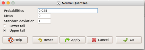
Figure 1. R Commander popup menu for Normal quantiles.
Thus, for our example, the 95% CI was ( ; our confidence in our estimate of the prevalence of diabetes in Hawaii is between 8.25% and 8.35%. Again, note that for our purposes it is OK to calculate the approximate confidence interval, replace with
 (for large N, the differences are observed in the 0.001 decimal).
Prevalence: R code
Rather than census counts, more likely we have results of smaller surveys. We use the epi.conf() function from the epiR package. Code adapted from example provided in epiR_descriptive vignette.
Note 1: Many R packages include vignettes, which, together with the package manual, is often helpful to understand what a function is intended to do and how to get the most from the function. R code to call all vignettes available for a package, eg, epiR:
vignette(package="epiR")
which will return names of available vignettes. For epiR, these are
epiR_descriptive Descriptive epidemiology (source, html)
epiR_surveillance Disease surveillance (source, html)
epiR_measures_of_association Measures of association (source, html)
epiR_sample_size Sample size calculations (source, html)
To call up the vignette we need for this example,
vignette("epiR_descriptive", package="epiR")
which brings up the page (assuming you installed the html help files during installation of base R).
library(epiR)
pop.Hawaii = 1.4e06
pop.Survey = 1000
type2.Survey = 80
Table.2 <- as.matrix(cbind(type2.Survey, pop.Survey))
epi.conf(Table.2, ctype = "prevalence", method = "exact", N = pop.Hawaii, design = 1, conf.level = 0.95) * 100
R output
   est    lower    upper
1    8 6.394198 9.857978
Thus, estimated Type 2 diabetes prevalence from the survey was 8, with 95% confidence interval 6.4 to 9.9 cases per 100 individuals. From 2020 U.S. Census, Hawai`i population was 1,455,271.
Note 2: Type 2 diabetes is one of many conditions for which prevalence is greater among Native Hawaiian and Pacific Islander populations compared to other groups in Hawai’i (Galinski et al 2016); these are called health disparitiess.
Incidence rate
Incidence of a disease (or condition) is defined as the occurrence of new cases of a disease. The simplest way to view incidence is that if everyone was followed for the same period of time, then incidence rate is the number of new cases since the start of the study divided by the total population. This is too simplistic, so we define a better metric called person-time. Incidence rate (IR) is then the ratio of the number of new cases divided by total person-time.
Again, incidence rate is an estimate. Therefore, we need a confidence interval. Assuming the population is large, then confidence interval can be calculated as

where IR is the incidence rate, T is the person-time, N is the number of events or cases, and z again is the standard normal probability (z ± 1.96 for 95% confidence interval).
For our example, N = 3 cases, T = 236 p-d, so 95% CI is (11.3%, 14.1%).
Person-time
Person-time can be days, months, years. Person-time is best defined with an example.
Five men join a study that will last 70 days. These men were selected because they had suffered a myocardial infarction (MI) and at the start of the study, they receive the same treatment. The outcome of the study is whether or not the subjects suffer a second MI.
The results are shown below
Subject A, 53 days
Subject B, 70 days
Subject C, 24 days
Subject D, 70 days
Subject E, 19 days
Add up the person days,

Now calculate the incidence rate,

that’s 3 cases (A, C, E) divided by 236 p-d = 0.0127. Multiply this by 1000 and we get our final answer for the incidence rate, 12.7 per person-days.
Incidence rate: R code
Incidence rate of myocardial infarction (MI) study. Code adapted from example provided in epiR_descriptive vignette.
ncas = 3
ntar = 236
tmp <- as.matrix(cbind(ncas, ntar))
epi.conf(tmp, ctype = "inc.rate", method = "exact", N = 1000, design = 1, conf.level = 0.95) * 1000
R output
          est    lower    upper
ncas 12.71186 2.621492 37.14946
The incidence rate of myocardial infarction was 12.7 (95% CI 2.6 to 37.2) cases per 1000 person-days.
Age-specific rates
Incidence or prevalence rates may be reported for specific age groups. For example, we can distinguish between number of live births in Hawaii in 2017, and numbers of live births by age group of the mother.
Age-adjusted rates
If populations with different age demographics, then the convention is to adjust the populations to a standard reference population with known age and other demographic properties. For example, the CDC uses the 2000 census as the standard population (CDC definitions, age adjustment, retrieved January 2023).
Questions
- Calculate the confidence interval of type 2 prevalence in Hawai`i with the 2020 census population value. How much did it change?
- Recalculate the confidence interval for a 99% confidence interval. Which estimate communicates greater confidence in the estimate?
Quiz
Quiz Chapter 7.2
Epidemiology basics
Chapter 7 contents
6.4 – Types of probability
Introduction
By probability, we mean a number that quantifies the uncertainty associated with a particular event or outcome. If an outcome is certain to occur, the probability is equal to 1; if an outcome cannot happen, the probability is equal to zero. Most events we talk about in biology have probability somewhere in between.
A basic understanding, or at least an appreciation for probability is important to your education in biostatistics. Simply put, there is no certainty in biology beyond simple expectations like Benjamin Franklin’s famous quip about “death and taxes…”
Discrete probability
You are probably already familiar with discrete probability. For example, what is the probability that a single toss of a fair coin will result in a “heads?” The outcomes of the coin toss are discrete, categorical, either “heads” or “tails.”
Note 1: Obviously, this statement assumes a few things — coin tossed not in a vacuum, for example. We assume a fair coin — equal chance heads or tails. Fair coins have two sides; tossing a coin we expect “heads” or “tails,” but rarely, some coin types may land and come to rest on edge or side (eg, USA nickels). We still consider the coin toss having binary outcomes, by definition, even though a coin may land on edge about one toss in six thousand (Murray and Teare 1993) because the exception is extremely rare. h/t Dr. Jerry Coyne.
And for ten tosses of the coin? And more cogently, what is the probability that you will toss a coin ten times and get all ten “heads?” While different in tone, these are discrete outcomes. An important concept is independence. Are the multiple events independent? In other words, does the toss of coin on the first attempt affect the toss of the coin on the second attempt and so on up to the tenth toss? At least in principle the repeated tosses are independent so to find the probability you just multiply each event’s probability to get the total.
In contrast, if one or more events are not independent but somehow influence the behavior of the next event, then you add the probabilities for each dependent event. We can do better than simply multiply or add events one at a time; depending on the number of discrete outcomes it is very likely that someone has already calculated all possible outcomes and come up with an equation. In the case of the tossing of two coins this is a binomial equation problem and repeat tosses can be modeled by use of the Bernoulli distribution.
Now, try this on for size. What is the probability that the next child born at Kapiolani Medical Center in Honolulu will be assigned female?
We just described a discrete random variable, which can only take on discrete or “countable” numbers. This distribution of values is the probability mass function. The probability of a one fatal airline accident in a year exactly on 20.1 is practically zero (the area under a point along the curve is zero), so we can get the probability of a range of values around the point as our answer.
Continuous probability
Many events in biology are of degree, not kind. It is kind of awkward to think about it, but for a sample of adult house mice drawn from a population, what is the probability of obtaining a mouse that is 20.0000 grams (g) in weight? Each possible value of body mass for a mouse is considered an event, just like in our example of tossing a coin. But clearly, we don’t expect to get a lot of mice that are exactly 20.0000 g in weight. For variables like body mass, the type of data we collect is continuous, and the probability values need to be rethought along a continuum of possible values and, in turn, how likely each value is for a mouse. Although it is theoretically possible that a mouse could weigh ten pounds, we know by experience that this is impossible. Adult mice weigh between 15 and 50 g or there about.
We just described a continuous random variable, which can take on any value between a specific interval of values. This distribution of values is the probability density function (PDF). The probability of a mouse’s weight falling exactly on 20.1 is practically zero (the area under a point along the curve is zero), so we can get the probability of a range of values around the point as our answer.
In statistical inference, following our measurements of the variables from our sample drawn from a population, we make conclusions with the following kind of caveat: “the mean body mass for this strain of mouse is 20 g.” That is our best estimate of the mean (middle) for the population of mice, more specifically, for the body mass of the mice. Here, the variable body mass is more formally termed a random variable. This implies that there is in fact a true population mean body mass for the mice and that any deviations from that mean are due to chance.
In statistics we don’t settle for a single point estimate of the population mean. You will find most reporting of estimates of random variables is accompanies by a statement like, the mean was 20g with a 95% probability that the true population mean is between 18.9 and 21 g. This is called the 95% confidence interval for the mean and it takes into account how good of an estimate our sample is likely to be relative to the true population value. Not only are we saying that we think the population mean is 20g, but we’re willing to say that we are 95% certain that the true value must be between a lower limit (18.9 g) and and upper limit (21 g). In order to make this kind of statement we have to assume a distribution that will describe the probability of mouse weights. For many reasons we usually assume a normal distribution. Once we make this assumption we can calculate how probable a particular weight is for a mouse.
We introduced how to calculate Confidence Intervals in Chapter 3.4 and will extend this in any chapter that introduces an estimation.
Types of probability
To begin refining our concept of probability, it is sometimes useful to distinguish among kinds of probabilities:
- between theoretical and empirical;
- between subjective and objective.
In most cases, including your statistics book, we would begin our discussion of probability by talking of some probabilities for events we’re familiar with.
- The theoretical probability of heads appearing the next time you flip a fair coin is 1/2 or 50%. As long as we’re talking about a fair coin, the probability of a heads appearing each time you flip the coin remains 50%. We can check this by conducting and experiment: out of 10 tosses, how many heads appear? The answer would be an empirical probability, and we understand the chance in an objective manner (no interpretation needed).
- The theoretical probability that a “5” will appear on the face of a fair dice after a toss is 1/6 or 16.667%. Again, as long as we’re talking about a fair dice, the probability of a “5” appearing each time you roll the dice remains 16.667%.
- The probability that at birth, a human baby’s sex will be male about 1/2 or 50%. This is an empirical probability based on millions of observations. Changes in technology, and ethical standards notwithstanding, the probability will remain the same.
- The probability of the birth of a Downs syndrome baby is 1/800, but increases with age until by age 45, the chance is 1/12. Again, these are empirical and objective.
- The probability of winning the Publisher’s Clearing House Sweepstakes is about 1 in 100 million. This probability is theoretical, it is also objective; however, by adding lots of twists to the game, by having multiple opportunities and by giving the appearance that a person must purchase a magazine, some players perceive their chances as increasing or decreasing by their efforts (=subjective).
R and distributions
R offers access to many named distributions. R generally provides four functions available for each.
density (d):the probability density function (PDF) for continuous distributions or the probability mass function (PMF) for discrete distributions.
probability (p): the cumulative distribution function (CDF), which is the chance (probability) of a random variable being less than or equal to a given value
quantile (q): the quantile function (inverse CDF), which returns the value at a given probability
r: draw random numbers from the specified distribution.
Examples of functions for the normal distribution then, are: dnorm(), pnorm(), qnorm(), and rnorm().
Coding example: Find the PDF for x = 0 in a standard normal distribution. # Find the PDF value for x = 0 in a standard normal distribution (mean=0, sd=1)
dnorm(x = 0, mean = 0, sd = 1)
R output
0.398942280401433
Thus, we conclude the chance that x = 0 is about 40%.
Note 2: Technically it’s not the chance that x is exactly 0 — it refers to the chance that the random variable falls within fractionally small interval around that value. That’s the calculus foundation for probability speaking.
Coding example: Find the probability that for x is equal to -1.2 or less in a standard normal distribution.
pnorm(q = -1.2, mean = 0, sd = 1, lower.tail = TRUE)
R output
0.115069670221708
Thus, we conclude the chance that x is equal to or less than -1.2 is about 11.5%.
Coding example: Assuming normal distribution of test scores, what score will 50% of students score? Find the probability that for x is equal to -1.2 or less in a standard normal distribution.
qnorm(0.5, mean = 75, sd = 10)
R output
75
As expected, at 50% it returns the mean. Now, confirm that the lower 25% and upper 75% are 68.26 and 81.75, respectively.
Last coding example, draw random sample of three scores from the same exam.
rnorm(3, mean = 75, sd = 10)
R output
-
66.0384856946112
-
69.1887923903669
-
77.6342297053815
R Commander: Distributions menus give four options
- Quantiles
- Probabilities
- Plot
- Sampling
Note 3: Looking for more examples? These kinds of problems are common skill-based questions one finds in any statistics course. Homework 3: Distributions & Probability in Mike’s Workbook for Biostatistics offers several additional examples to work through. Additional examples are provided in Chapter 6.5 and Chapter 6.6.
Questions
1. Define and distinguish, with examples
- discrete and continuous probability
- theoretical and empirical probability
- subjective and objective probability
Quiz Chapter 6.4
Types of probability
Chapter 6 contents
- Introduction
- Some preliminaries
- Ratios and proportions
- Combinations and permutations
- Types of probability
- Discrete probability distributions
- Continuous distributions
- Normal distribution and the normal deviate
- Moments
- Chi-square distribution
- t distribution
- F distribution
- References and suggested readings