3.5 – Statistics of error
Making sense of error in data.
This page explains how statistics of error help quantify differences between measured and true values, beginning with classical methods like standard error and confidence intervals that rely on large-sample assumptions. Related, statisticians talk about uncertainty — the quantification of doubt about a measurement. We introduce permutation-based approaches, including jackknife and bootstrap resampling, which avoid those assumptions and are especially useful with smaller or complex data sets. Observer variation (intra- and interobserver error) is also highlighted as an important source of measurement error.
Missing values are another common source of uncertainty in biological data sets. Data may be missing because of equipment failure, recording mistakes, sample loss, or biological factors that prevent a measurement from being collected. Even a small number of missing observations can influence summaries, graphs, and statistical tests, especially in smaller studies. In this chapter, we treat missing values mainly as a practical issue to identify and report during exploratory data analysis. Later, in the chapter on experimental design, we examine missing data in greater depth, including differences between random and non-random missingness, as well as approaches such as data imputation and the consequences these choices may have for interpretation.
We conclude with a discussion about confidence intervals as a measure of accuracy and emphasize proper use of significant figures to avoid overstating precision.
Statistics of error.
In statistics, error doesn’t mean mistake, an avoidable human misjudgement or oversight, eg, a typo. An error in statistics means there was a difference between the measured value and the actual value for an object. Efforts by many authors of notable classical statistics developed a large body of calculated statistics, eg, standard error the mean, which allows the user to quantify how large the error of measurement is given assumptions about the distribution of the errors. Thus, classical statistics requires user to make assumptions about the error distribution, the subject of our Chapter 6. A critical issue to understand is that these methods assume large sample sizes are available; they are called asymptotic statistics or large-sample statistics; the properties of the statistical estimates are evaluated as sample size approaches infinity.
Jackknife sampling and bootstrap sampling are permutation approaches to working with data when the Central Limit Theorem — as sample size increases, the distribution of sample means will tend to a normal distribution (see Chapter 6.7) — is unlikely to apply or, rather, we don’t wish to make that assumption (Chapter 19). The jackknife is a sampling method involving repeatedly sampling from the original data set, but each time leaving one value out. The estimator, for example, the sample mean, is calculated for each sample. The repeated estimates from the jackknife approach yield many estimates which, collected, are used to calculate the sample variance. Jackknife estimators tend to be less biased than those from classical asymptotic statistics.
Bootstrapping, and not jackknife resampling, may now be the preferred permutation approach (eg, Google Scholar search “bootstrap statistics” 36K hits; “jackknife statistics” 17K hits), but which method is best depends on qualities of the data set. Bootstrapping involves large numbers of permutations of the original data, which, in short, means we repeatedly take many samples of our data and recalculate our statistics on these sets of sampled data. We obtain statistical significance by comparing our result from the original data against how often results from our permutations on the resampled data sets exceed the originally observed results. By permutation methods, the goal is to avoid the assumptions made by large-sample statistical inference, ie, reaching conclusions about the population based on samples from the population. Since its introduction, “bootstrapping” has been shown to be superior in many — but, importantly, not all — cases for statistics of error compared to the standard, classical approach (Efron 1979, Hesterberg 2015).
There are many advocates for the permutation approaches, and, because we have computers now instead of the hand calculators our statistics ancestors used, permutation methods may be the approach you will take in your own work. However, the classical approach has its strengths — when the conditions, that is, when the assumptions of asymptotic statistics are met by the data, then the classical approaches tend to be less conservative than the permutation methods. By conservative, statisticians mean that a test performs at the level we expect it to. Thus, if the assumptions of classical statistics are met they return the correct answer more often than do the permutation tests.
Error and the observer.
Individual researchers make observations, therefore, we can talk about observer variation as a kind of error measurement. For repeated measures of the same object by an individual, we would expect the individual to return the same results. To the extent repeated measures differ, this is intraobserver error. In contrast, measures of the same object from different individuals is interobserver error. For a new instrument or measurement system, one would need to establish the reliability of the measure: confronted with the same object do researchers get the same measurement? Accounting for interobserver error applies in many fields, eg, histopathology of putative carcinoma slides (Franc et al 2003), liver biopsies for cirrhosis (Rousselet et al 2005), blood cell counts (Bacus 1973).
Confidence in estimates.
A really useful concept in statistics is the idea that you can assign how confident you are to an estimate. This is another way to speak of the accuracy of an estimate. Clearly, we have more confidence in a sample estimate for a population parameter if many observations are made. Another factor in our ability to estimate is the magnitude of observation differences. In general, the larger the differences among values from repeated trials, the less confident we will be in out estimate, unless, again, we make our estimates from a large collection of observations. These two quantities, sample size and variability, along with our level of confidence, eg, 95%, are incorporated into a statistic called the confidence interval.

We will use this concept a lot throughout the course; for now, a simple but approximate confidence interval is to use the 2 x SEM rule (as long as sample size large): twice the standard error of the mean. Take your estimate of the mean, then add (upper limit) or subtract (lower limit) twice the value of the standard error of the mean (if you recall, that’s the standard deviation divided by the square-root of the sample size).
Example. Consider five magnetic darts thrown at a dart board (28 cm diameter, height of 1.68m from the floor) from a distance of 3.15 meters (Fig 1).

Figure 1. Magnetic dart board with 5 darts. Click image to view full sized image.
The distance in centimeters (cm) between where each of the five darts landed on the board compared to the bullseye is reported in (Table 1),
Table 1. Results of five darts thrown at a target (Figure 2)*
| Dart | Distance |
|---|---|
| 1 | 7.5 |
| 2 | 3.0 |
| 3 | 1.0 |
| 4 | 2.7 |
| 5 | 7.4 |
* distance in centimeters from the center.
Note 1: Use of the coordinate plane, and including the angle measurement in addition to distance (the vector) from center, would be a better analysis. In the context of darts, determining accuracy of a thrower is an Aim-Point targeting problem and part of your calculation would be to get MOA (minute of angle). For the record, the angles (degrees) were
| Dart | Distance | Angle |
|---|---|---|
| 1 | 7.5 | 124.4 |
| 2 | 3.0 | -123.7 |
| 3 | 1.0 | 96.3 |
| 4 | 2.7 | -84.3 |
| 5 | 7.4 | -31.5 |
measured using imageJ. Because there seems to be an R package for just about every data analysis scenario, unsurprisingly, there’s an R package called shotGroups to analyze shooting data.
How precise was the dart thrower? We’ll use the coefficient of variation as a measure of precision. Second, how accurate were the throws? Use R to calculate
darts = c(7.5, 3.0, 1.0, 2.7, 7.4)
#use the coefficient of variation to describe precision of the throws
coefVar = 100*(sd(darts)/mean(darts)); coefVar
[1] 68.46141
Confidence Interval to describe accuracy.
For a game of darts, the true value would be a distance of zero — all bullseyes. We need to calculate the standard error of the mean (SEM), then, we calculate the confidence interval around the sample mean.
#Calculate the SEM
SEM <- sd(darts)/sqrt(length(darts)); SEM
[1] 1.322649
#now, get the lower and upper limit, subtract from the mean
confidence <- c(mean(darts)-2*SEM, mean(darts), mean(darts)+2*SEM); confidence
[1] 1.674702, 4.320000, 6.965298
The mean was 4.3 cm, therefore to get the lower limit of the interval subtract 2.65 (2*SEM = 2.645298) from the mean; for the upper limit add 2.65 to the mean. Thus, we report our approximate confidence interval as (1.7, 7.0), and we read this as saying we are about 95% confident the population value is between these two limits. Five is a very small sample number, so we shouldn’t be surprised to learn that our approximate confidence interval would be less than adequate. In statistical terms, we would use the t-distribution, and not the normal distribution, to make our confidence interval in cases like this.
Note 2: As a rule, implied by Central Limit theory and use of asymptotic statistical estimation, a sample size of 30 or more is safer, but probably unrealistic for many experiments. This is sometimes called as the rule of thirty. (For example, a 96-well PCR array costs about $500; with n = 30, that’s $15,000 US Dollars for one group!). So, what about this rule? This type of thinking should be avoided as “a relic of the pre-computer era,” (Hesterberg, T. (2008). It’s Time To Retire the” n>= 30″ rule.). We can improve on asymptotic statistics by applying bootstrap principles (Chapter 19).
We made a quick calculation of the confidence interval; we can get make this calculation by hand by incorporating the t distribution. We need to know the degrees of freedom, which in this case is 4 (n – 1, where n = 5). We look up critical value of t at 5% (to get our 95% confidence interval), t = 2.78. Subtract for lower limit t*SEM and add for upper limit t*SEM to the sample mean for the 95% confidence interval.
We can get help from R, by using the one-sample t-test with a test against the hypothesis that the true mean is equal to zero. Among a variety of output we will introduce later (see Chapter 8 and 10), the confidence interval is reported (yellow highlight),
#make an attach a data frame object
Ddarts <- data.frame(darts)
t.test(darts,mu=0)
One Sample t-test
data: darts
t = 3.2662, df = 4, p-value = 0.0309
alternative hypothesis: true mean is not equal to 0
95 percent confidence interval:
 0.6477381 7.9922619
sample estimates:
mean of x
 4.32
t.test uses the function qt(), which provides the quantile function. To recreate the 95% CI without the additional baggage output from the t.test, we would simply write
#upper limit
mean(darts)+ qt(0.975,df=4)*sd(darts)/sqrt(5)

#lower limit
mean(darts)+ qt(0.025, df = 4, lower.tail=TRUE)*sd(darts)/sqrt(5)
where sd(darts)/sqrt(5) is the standard error of the mean.
Or, alternatively, download and take advantage of a small package called Rmisc (not to be confused with the RcmdrMisc package) and use the function CI
library(Rmisc)
CI(darts)
     upper     mean     lower
7.9922619 4.3200000 0.6477381
The advantage of using the CI() command from the package Rmisc is pretty clear; I don’t have to specify the degrees of freedom or the standard error of the mean. By default, CI reports the 95% confidence interval. we can specify any interval simply by adding to the command. For example,
CI(darts, ci=0.90)
reports upper and lower limits for the 90% confidence interval.
Try it. On your own, get the 90% confidence interval and the 99% confidence intervals for our dart example. Compare to the 95% confidence interval — what do you conclude about “confidence” in our estimate from 90% to 99%?
Confidence intervals from p-values.
And finally, it is not unusual for a report to provide summary statistics, differences between means (ie, effect size), and p-values (orange highlight), but not report confidence intervals. We discuss p-values and the concept of statistical significance beginning in Chapter 8. But for now, we show how to calculate approximate confidence intervals from the p-value. This may be of use for conducting meta-analysis (Chapter 20.15). See two helpful “how to” articles by Bland and Altman in 2011 BMJ (references listed in Chapter 3.6 – References).
In brief, calculate the test statistic for a normal distribution (letZ), calculate a standard error, and then the lower and upper limits for the 95% confidence interval. We illustrate use of the calculator formulas with the dart example, the p-value was 0.0309; the estimate was 4.32.
R code
letZ = (-0.862 + sqrt(0.743 - 2.404*log(0.0309, base = exp(1)))) = 2.154903
letSE = 4.32/letZ = 2.00473
1.96*letSE = 3.929271 # Add for upper and subtract for lower
The lower limit is 0.39 (4.32 – 3.929271) and the upper limit is 8.25 (4.32 + 3.929271). Although in the ballpark, these calculated estimates are wider than the confidence interval estimated by the t.test command. Small sample size, n = 5, is to blame — the accuracy of these methods, based on asymptotic statistical estimation approaches, assumes the law of large numbers applies.
Significant figures.
And finally, we should respect significant figures, the number of digits which have meaning. Our data were measured to the nearest tenth of a centimeter, or two significant figures. Therefore, if we report the confidence interval as (0.6477381, 7.9922619), then we imply a false level of precision, unless we also report our random sampling error of measurement.
R has a number of ways to manage output. One option would be to set number of figures globally with the options() function — all values reported by R would hold for the entire session. For example, options(digits=3) would report all numbers to three significant figures. Instead, I prefer to use signif() function, which allows us to report just the values we wish and does not change reporting behavior for the entire session.
signif(CI(darts),2)
upper  mean lower
 8.00  4.30  0.65
Note 3: The options() function allows the R user to set a number of settings for an R session. After gaining familiarity with R, the advanced user recognizes that many settings can be changed to make the session work to report in ways more convenient to the user. If curious, submit options() at the R prompt and available settings will be displayed.
The R function signif() applies rounding rules. We apply rounding rules when required to report estimates to appropriate levels of precision. Rounding procedures are used to replace a number with a simplified approximation. Wikipedia provides a comprehensive list of rounding rules. Notable rules include
- directed rounding to an integer, eg, rounding up or down
- rounding to nearest integer, eg, round half up (down) if the number ends with 5
- randomly rounding to an integer, eg, stochastic rounding.
With the exception of stochastic rounding, all rounding methods impose biases on the sets of numbers. For example, the round half up method applied for numbers above 5, round down for numbers below 5 will increase the variance of the sample. In R, use round() for most of your work. If you need one of the other approaches, for example, to round up, the command is ceiling(); to round down we use floor().
When to round?
No doubt your previous math classes have cautioned you about the problems of rounding error and their influence on calculation. So, as a reminder, if reporting calls for rounding, then always round after you’ve completed your calculations, never during the calculations themselves.
A final note about significant figures and rounding. While the recommendations about reporting statistics are easy to come by (and often very proscriptive, eg, Table 1, Cole 2015), there are other concerns. Meta-analysis, which are done by collecting information from multiple studies, would benefit if more and not fewer numbers are reported, for the very same reason that we don’t round during calculations.
Questions
- Calculate the correct 90% and 99% confidence intervals for the dart data using the t-distribution
- by hand
- by one alternative method in R, demonstrated with examples in this page
- How many significant figures should be used for the volumetric pipettor p1000? The p200? The p20 (data at end of this page)?
- Another function,
round(), can be used. Try
round(CI(darts),2)
-
- and report the results: vary the significant figures from 1 to 10 (
signif()will take digits up to 22). - See any output differences between
signif()andround()? Don’t forget to take advantage of R help pages (eg, enter?roundat the R prompt) and see Wikipedia.
- and report the results: vary the significant figures from 1 to 10 (
- Compare rounding by
signif()andround()for the number 0.12345. Can you tell which rounding method the two functions use? - Calculate the coefficient of variation (CV) for each of the three volumetric pipettors from the data at end of this page. Rank the CV from smallest to largest. Which pipettor had the smallest CV and would therefore be judged the most precise?
- (data provided at end of this page, click here).
- Standards distinguish between within run precision and between run precision of a measurement instrument (see Chapter 16.5 – Instrument reliability and validity). The data in Table 1 were all recorded within 15 minutes by one operator. What kind pf precision was measured?
- Calculate the standard error of the means for each of the three pipettors from the data
- (data provided at end of this page, click here).
- Calculate the approximate confidence interval using the 2SE rule and judge which of the three pipettors is the most accurate (narrowest confidence interval)
- Repeat, but this time apply your preferred R method for obtaining confidence intervals.
- Compare approximate and R method confidence intervals. How well did the approximate method work?
- Return to the dart example, but now assume the p-value was p = 0.003 and again for p = 0.0003. Estimate the 95% confidence interval for each case; the difference remains 4.32. How does the change in p-value, from 0.03 to 0.0003 — a two orders of magnitude difference — affect the estimates for the confidence interval (hint: describe the width of the CI)?
Quiz Chapter 3.5
Statistics of error
Data sets
Pipette calibration
| p1000 | p200 | p100 |
|---|---|---|
| 0.113 | 0.1 | 0.101 |
| 0.114 | 0.1 | 0.1 |
| 0.113 | 0.1 | 0.1 |
| 0.115 | 0.099 | 0.101 |
| 0.113 | 0.1 | 0.101 |
| 0.112 | 0.1 | 0.1 |
| 0.113 | 0.1 | 0.1 |
| 0.111 | 0.1 | 0.1 |
| 0.114 | 0.101 | 0.101 |
| 0.112 | 0.1 | 0.1 |
Chapter 3 continues
19 – Distribution free statistical methods
Introduction
We introduced the concept of permutation tests in our chapter on parameter estimates and statistical error (Chapter 3.3). Jackknife and bootstrapping are permutation approaches to working with data when the Central Limit theorem is unlikely to apply or, rather, we don’t wish to make that assumption. The jackknife is a sampling method involving repeatedly sampling from the original data set, but each time leaving one value out. The estimator, for example, the sample mean, is calculated for each sample. The repeated estimates from the jackknife approach yield many estimates which, collected, are used to calculate the sample variance. Jackknife estimators tend to be less biased than those from classical asymptotic statistics. Bootstrapping, and not jackknife resampling, is now the preferred permutation approach (add citations).
Bootstrapping
Bootstrapping involves large numbers of permutations of the data, which, in short, means we repeatedly take many samples of our data and recalculate our statistics on these sets of sampled data. We obtain statistical significance by comparing our result from the original data against how often results from our permutations on the resampled data sets exceed the originally observed results. By permutation methods, the goal is to avoid the assumptions made by large-sample statistical inference. Since its introduction, “bootstrapping” has been shown to be superior in many cases for statistics of error compared to the standard, classical approach (add citations).
Permutation vs classical NHST approach
There are many advocates for this approach, and, because we have computers now instead of the hand calculators our statistics ancestors used, permutation methods may be the approach you will take in your own work. However, the classical approach has it’s strengths; when the conditions, that is, when the assumptions of asymptotic statistics are met by the data, then the classical approaches tend to be less conservative than the permutation methods. By conservative, statisticians mean that a test performs at the level we expect it to. Thus, if the assumptions of classical statistics are met they return the correct answer more often than do the permutation tests.
Questions
[pending]
Chapter 19 contents
13.2 – Why tests of assumption are important
Introduction
Note that R (and pretty much all statistics packages) will calculate t-tests or ANOVA or whatever test you ask for, and return a p-value, but it is up to you to recognize that the p-value is accurate only if the assumptions are met. Thus, you can always estimate a parameter, but interpret its significance (biological, statistical) with caution. The great thing about statistics is that you can directly evaluate whether assumptions hold.
Violation of the assumptions of normality or equal variances can lead to Type I errors occurring more often than the 5% level. That means you will reject the null hypothesis more often than you should! If the goal of conducting statistical tests on results of an experiment is to provide confidence in your conclusions, then failing to verify assumptions of the test are no less important than designing the experiment correctly in the first place. Thus, the simple rule is: know your assumptions, test your assumptions. Evaluating assumptions is a learned skill:
- Conduct proper data exploration.
- Use specialized statistical tests to evaluate assumptions.
- data normally distributed? eg, histogram, Shapiro-Wilk test.
- groups equal variance? eg, box-plot, Levene’s median test.
- Evaluate influence of any outlier observations.
What to do if the assumptions are violated?
This is where judgement and critical thinking apply. You have several options.
First, if the violation is due to only a few observations, then you might proceed anyway, in effect invoking the Central Limit Theorem as justification.
Second, you could check your conclusions with and without the few observations that seem to depart from the trend in the rest of the data set — if your conclusion holds without the “outliers”, then you might conclude that your results are robust).
Third, you might apply a data transform reasoning that the distribution from which the data were sampled was log-normal, for example. Applying a log transform (natural log, base 10, etc,) will tend to make the variances less different among the groups and may also improve normality of the samples.
Fourth, if the violated assumption involves variances differ across different groups or levels of the factors or predictors, then there are more sophisticated alternatives, including use of Generalized Linear Models and creating a model to capture the relationship between predictor means and variances. Additionally, Weighted Least Squares (WLS) can be employed, giving more weight to observations with smaller variances.
Fifth, if a nonparametric test is available, you might use it instead of the parametric test. For example, we introduced the Levene’s test of equal variances as a better choice than the parametric F test. Additionally, there are many nonparametric alternatives to parametric tests. For example, t-tests are parametric and their non-parametric alternatives include tests like Wilcoxon and Mann-Whitney. ANOVA, too is parametric, and its nonparametric alternative version is called rank ANOVA (see also Kruskal-Wallis). See Chapter 15 for nonparametric tests.
Finally, a resampling approach could be taken, where the data themselves are used to generate all possible outcomes like the Fisher Exact test; with large sample size, bootstrap or Jackknife procedures are used (Chapter 19).
For now, let’s introduce you to the kinds of nonparametric statistical tests for which the t-test is just one example. For the independent sample t-test, our first method to account for the possible violation of equal variances is a parametric test, Welch’s variation of the Student’s t-test. Instead of the pooled standard deviation, Welch’s test accounts for each group’s variance in the denominator.
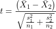
The degrees of freedom for the Welch’s test are now
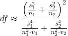
where df for Student’s t-test was  . Note that Welch’s test assumes normal distributed data.
Note 1: In R and therefore R Commander, the default option for conducting the t-test is Welch’s version, not the standard t-test (Fig 1).
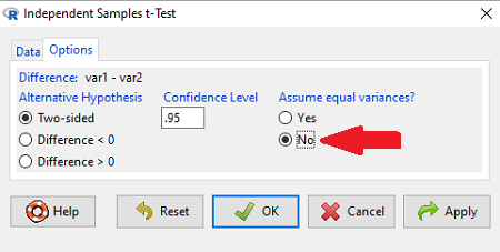
Figure 1. Screenshot of Rcmdr options menu for independent t-test. Red arrow points to default option “No,” which corresponds to Welch’s test.
See discussions in Olsen (2003), Choi (2005), and Hoekstra et al (2012).
How to report choices made about data transformations?
Eventually, with all of the analysis completed, one has to decide what to report. We touched on How to Report Statistics in Chapter 4. However, that chapter emphasized a balance between reporting results in sentences, tables, or as graphics. Here, we need to emphasize a different quality about reporting of statistical methods, that is, transparency. In both reporting contexts — how to report the results and how to report any data transformations — the goal is to provide sufficient detail so that the reader can follow (reproducibility criteria). If guidance presented on Chapter 13.1 and on this page is taken literally, there would seem to be a nearly endless number of graphs and statistical results to report. Clearly, this can’t be the answer.
For students in BI311 there should be clear guidance for what is expected for reporting in homework. More generally, when analysis leads to a completed project ready for reporting at conference or as a journal article, then the goal is to provide enough information so that the reader can evaluate the choices you made.
Consider the body mass data presented on this page. Results of various tests on both raw and log10-transformed data were provided. The context was check of normality assumption, and, based on the results we should conclude that the log10-transformed data better achieved the assumption of normality. Therefore, we would not report all the figures from Chapter 13.1: Figure 2, Figure 3, Figure 4, Figure 5, and Figure 6. I would report only Figure 2 — the raw data– with a few sentences: “The data were log10-transformed to address violations of normality assumption. Normality was assessed by calculation of the moment statistics skewness and kurtosis and Q-Q plots. All subsequent tests were conducted on the log10-transformed data set.” I wouldn’t report the exact results of the Q-Q plots or the moment statistics, but would include names or references to the specific tests used.
Note 2: Log10-transform would also likely improve unequal variances. Therefore, I would need to modify my sentences to account for this, eg, “The data were log10-transformed to address violations of normality and equal variance assumptions.”
Questions
Please skim read articles about statistical assumptions for common statistical tests:
- Choi (2005), click link to article.
- Hoekstra et al. (2012), click link to article.
- Olsen (2003), click link to article.
From the articles and your readings in Mike’s Biostatistics Book, answer the following questions
- What are some consequences if a researcher fails to check statistical assumptions?
- Explain why use of graphics techniques may be more important than results of statistical tests for checks of statistical assumptions.
- Briefly describe graphical and statistical tests of assumptions of (1) normality and (2) equal variances
- Pick a biological research journal for which you have online access to recent articles. Pick ten articles that used statistics (eg, look for “t-test” or “ANOVA” or “regression”; exclude meta analysis and review articles — stick to primary research articles). Scan the Methods section and note whether or not you found a statement that confirms if the author(s) checked for violation of (1) normality and (2) equal variances. Construct a table.
- Review your results from question 3. Out of the ten articles, how many reported assumption checking? How does your result compare to those of Hoekstra et a; (2012)?
Quiz Chapter 13.2
Why tests of assumption are important
Chapter 13 contents
- Introduction
- ANOVA Assumptions
- Why tests of assumption are important
- Test assumption of normality
- Tests for Equal Variances
- References and suggested readings
11.3 – Factors influencing statistical power
Introduction
Components of an experimental design that may influence statistical power include:
- α (probability of committing a Type I error).
As the probability of a Type I error increases, the probability of a Type II error decreases. Therefore, as α gets bigger, power gets decreases. - σ, the variance in the population
Statistical power decreases as variability increases. - Effect size
The effect size is a measure of the differences between two or more groups considered biologically important; its difficult to have lots of power to detect very small differences. - Sample size
As n increases, power increases
Size of alpha (Type I error)
When we introduced the idea of Type I error, alpha, it followed a story about Challenger, the space shuttle that disintegrated after failure of O-rings allowed hot gasses to cross joints in the rockets. If we adopt a Type I error rate of 5% in our rocket designs, then failure is expected at one in twenty launches. That rate clearly is unacceptable, so the logical extension of this thinking would be to decrease the Type I error rate. Unfortunately, this comes at the expense of increasing our risk of Type II error. Thus, decreasing Type I error decreases statistical power.
Variance
If the range of values for individuals in the samples are great, then it should not be surprising that the power to distinguish between sample means from the groups will be low. Conversely, if the variance for a sample is small, then the precision of the estimated sample mean will increase, and, therefore, the power will increase.
Effect size
Effect size deserves some more comments. If we are thinking cause/effect, then we are asking whether or not our independent variable explains a lot of variation in the response (dependent) variable. If there is a strong link between the independent and dependent variable, then the effect size will be large and small numbers of observations will be needed.
There are various ways to estimate effect size, but the simplest is a variation of the t-test (Cohen’s d).

The formula would be different for ANOVA (involves the mean squares), but you get the idea. By convention, an effect size of about 0.2 would be “small,” 0.5 would be “medium,” and an effect size greater than 0.8 would be “large.”
Sample size
This is the area of course where the experimenter has control. We can choose how many individuals are assigned to treatment groups. The Central Limit Theorem basically states that you can use the normal distribution to predict how likely an individual observation is in relation to a sample mean even if the sample distribution is not normally distributed. The larger the number of individuals in the sample from a population, the more confidence we have about making this assumption. Translation: sample size directly impacts standard error of the calculated statistic. Recall our equation for the standard error of the mean.
Alternatives to Cohen’s d
Glass’s g
Hedges’ gu
Keselman and colleagues’ dj
estimators based on trimmed mean and Winsorized variances.
Questions
- The Central limit Theorem can be invoked when we have large samples of observations. In this subchapter we state that increase sample size increases statistical power. Discuss and contrast these two characteristics of large sample size on statistical inference.
- How many samples are enough? Some statistical textbooks will cite a rule of 30. With respect to factors that affect statistical power, discuss the limitations of adopting such a rule to design an experiment.
Quiz Chapter 11.3
Factors influencing statistical power
Chapter 11 contents
- Introduction
- What is Statistical Power?
- Prospective and retrospective power
- Factors influencing statistical power
- Two sample effect size
- Power analysis in R
- References and suggested readings
7.6 – Confidence intervals
Quantifying uncertainty.
Although I’ve already presented the concept (eg, Chapter 3.4), and equations for confidence intervals of risk estimates (Chapter 7.4, Chapter 7.5), here, we expand on the idea of confidence intervals. Confidence intervals are a central part of meeting one of the main objectives of statistics, that is, estimation and communicating uncertainty with any reported estimate.
There are three components of statistical analysis
- Estimation
- Inference
- Modeling
Inference refers to statistical hypothesis testing — we ask questions of observations — do men (Rice et al 1999) and women (Fisher et al 2012) differ for blood glucose levels following a bout of aerobic exercise? T-tests, analysis of variance (ANOVA), chi-square, correlation, regression are types of statistical procedures used to do statistical inference. Modeling on the other hand refers to procedures used to relate cause and effect or for use in prediction of future values given new data. Many of the statistical procedures one uses for inference are also used to build statistical models (ANOVA, regression). Studies may intend to either test some hypothesis (inference) or to provide a predictive equation (modeling). But most studies that relate observations gathered from an experiment are obliged to also report statistics, and this is the realm of estimation. Estimates of the mean and standard deviation, for example, would be typical statistics one expects to find in a report. We call these descriptive statistics, and together with graphics, descriptive statistics are the chief way we describe our results.
Confidence intervals are crucial in statistics because they provide a range of values where the true population parameter is likely to fall, offering a more nuanced understanding of the estimate beyond just a single point value. Similarly, for statistical model model building, confidence intervals quantify the uncertainty inherent in data, providing a range of plausible values for model parameters rather than a single point estimate.
We will review how to calculate confidence intervals for proportions and for NNT. These intervals are available in epiR package and automatically returned in RcmdrPlugin.EBM.
Confidence interval for proportions
A proportion is the fraction of individuals in a population with some characteristic. The characteristic might be HIV positive for example. This would be called the population proportion and it would be a parameter of interest. In reality, we calculate a sample proportion and therefore estimate the population proportion with error. We can calculate the confidence interval (CI) of the proportion to communicate the precision of our estimate. For proportions, we use the binomial distribution — either a sample has the characteristic of interest or it does not — there are only two possibilities. There are a variety of ways to go here, and the simplest is to use a normal approximation. This will work well provided the sample size was reasonably large and the proportion is not close to zero or one, that is, we invoke the Central Limit Theorem here. Although the outcomes are binomial, the error is assumed to be normally distributed. The Wald confidence interval for p is

where  is the proportion of individuals with the characteristic (also called successes), z is the percentile from the normal distribution that corresponds to 1 – 1/2α. For 95% CI then α = 0.05 and z would be 1.965. (See standard normal table.) Of course, if making the normal approximation for the binomial is not appropriate, the CI is less than ideal. The binomial after all is a discrete distribution whereas the normal distribution is continuous, so errors will enter particularly for low sample numbers.
Other approaches may be used to get better estimates of CI for proportions, including Wilson score intervals and Jeffrey Intervals (Agresti and Coull 1998). See R package propCIs.
Because a statistic like the mean or a calculation of absolute or relative risk reduction are calculated from samples drawn from a population, the estimate comes with error. The error is basically this – if we calculate a statistic like number needed to treat (NNT) or its converse, the number needed to harm (NNH), we need to communicate to the reader how precise our estimate is. Estimation has to do with accuracy, error, and precision.
Confidence interval for ARR
The ARR is simply 
where  is the number of treated or exposed individuals for which the event occurred and
 is the number of untreated or unexposed individuals which the event occurred.
| Event happened | Event did not happen | |
| Treated or Exposed |
a | b |
| Control or Not exposed |
c | d |
Our data from example (Ch 7.5), were a = 612, b = 2192, c = 375, and d = 2543.

and the 95% confidence interval is then 
approximately. The “2” is only approximate; you need to use Z = 1.965, the value at probability value = 0.9725 (which comes from the Normal Table).
Confidence interval for NNT
For a sample of 100 people drawn at random from a population (which may number in the millions), then repeat the NNT calculation for a different sample of 100 people, do we expect the first and second NNT estimates to be EXACTLY the same number? No, but we do expect them to be close and we can define what we mean by close as we expect each estimate to be within certain limits. While we expect the second calculation to be close to the first estimate, we would be surprised if it was EXACTLY the same. And so, which is the correct estimate, the first or the second? They both are, in the sense that they both estimate the parameter NNT (a property of a population). But we can do better than two estimates. Confidence Intervals (CI) allow us to assign a probability to how certain we are about the statistic and whether it is likely to be close to the true value. We will
For CI of NNT, we need sample size for control and treatment groups; like all confidence intervals, we need to calculate the standard error of the statistic, in this, case, the standard error (SE) for NNT.
SE = sqrt(risk placebo * (1 - risk placebo) / (# in placebo group) + risk treatment * (1 - risk treatment) / (# in treatment group))
where SE is the standard error for NNT
The CI is approximately then 
* – the “2” is only approximate; you need to use Z = 1.965, the value at probability value = 0.9725 (by multiplying this, which comes from the Standard Normal Table).
Odds ratio Standard error and 95% confidence interval
Like any statistic we can calculate, an estimate of odds ratio should be accompanied by the confidence limit. The standard error may be calculated with the following formula

R code
seOdds <- sqrt(sum(1/612, 1/2192,1/375,1/2543))
where ln refers to the natural logarithm. An estimate for the 95% confidence interval is

where exp is the exponential function

and ln is natural logarithm.
R code
exp(log(1.89,base=exp(1)) - 1.96*seOdds)
Our example the lower limit was 1.64. For the upper limit

Our example the upper limit was 2.19.
R code
exp(log(1.89,base=exp(1)) + 1.96*seOdds)
Thus, our estimate was 1.89 and the 95% confidence interval was 
which does not include one. Therefore, we conclude statistically different.
Note 1. A reminder, log() without specifying the base returns the natural logarithm. A better coding habit might suggest always specifying the base:
log(x, base = exp(1))P-values from confidence intervals
While we expect certain reporting criteria for published, it is not uncommon that one or more elements are missing. For example, while we show how to obtain confidence intervals, the p-values were not reported. We discuss statistical inference and p-values in detail in Chapter 8, but for now, a low p-value (typically < 0.05) indicates that the odds ratio (OR) is statistically significant, meaning the observed relationship between a factor and an outcome is unlikely to be due to random chance. An OR of the difference may not be reported, or, an inexact p-value is reported like “< 0.05,” but we “need” an exact p-value for our meta-analysis. A little math, and these missing statistics can be calculated.
Note 2. We illustrated how to calculate confidence intervals from p-values in Chapter 3.4 – Estimating parameters. See two helpful “how to” articles by Bland and Altman in 2011 BMJ (references listed in Chapter 3.6 – References).
We can use the OR example. We need to take the logarithm of ratios like OR or NNT or RRR. From above, we have the confidence intervals.
We need
The OR estimate,  , which was 1.89
lower and upper confidence intervals: 1.64 and 2.19, respectively.
the standard error, which can be calculated as 
the test statistic, 
and then the p-value, 
we would then report that the OR was not statistically different, p = 0.4044).
Questions
1. Instead of 95% confidence interval, obtain the 99% confidence interval for odds ratio 1.89.
Quiz Chapter 7.6
Confidence intervals
Chapter 7 contents
6.6 – Continuous distributions
Large numbers and the Central Limit Theorem
Imagine we’ve collected (sampled) data from a population and now want to summarize the data sample. How do we proceed? A good starting point is to plot the data in a histogram and note the shape of the sample distribution. Not to get too far ahead of ourselves here, but much of the classical inferential statistics demands that we are able to assume that the sampled values come from a certain kind of distribution called the normal, or Gaussian distribution.
Consider a random sample drawn from a normally distributed population of the following series of graphs, Figures 1 – 4:
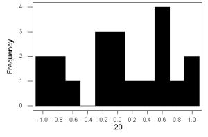
Figure 1. Sample size = 20, drawn from population with known μ = 0 and σ = 1.
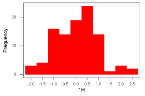
Figure 2. Sample size = 100, also drawn from population with known μ = 0 and σ = 1.
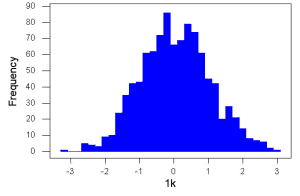
Figure 3. Sample size n = 1000, once again drawn from population with known μ = 0 and σ = 1.
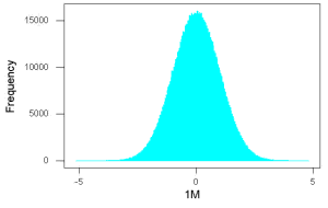
Figure 4. And lastly, sample size n = 1 million also drawn from population with known μ = 0 and σ = 1.
These graphs illustrate a fundamental point in statistics: for many kinds of measurements in biology, the more data you sample, the more likely the data will approach a normal distribution. This series of simulations was a quick and dirty “proof” of the Central Limit Theorem, which is one of the two fundamental theorems of probability, the other being that of Law of Large Numbers (ie, large-sample statistics). Basically the CLT says that for a large number of random samples, the sample mean will approach the population mean, μ, and the sample variance will approach the population variance σ2; the distribution of the large sample will converge on the normal distribution.
As the sample size gets bigger and bigger, the resulting sample means and standard deviations get closer and closer to the true value (remember — I TOLD the program to grab numbers from the Z distribution with a mean of zero and standard deviation = 1), obeying the Law of Large Numbers.
Simulation
I used the computer to generate sample data from a population. This process is called a simulation. R can make new data sets by sampling from known populations with specified distribution properties that we determine in advance — a very powerful tool — a technique used for many kinds of statistics (eg, Monte Carlo methods, bootstrapping, etc., see Chapter 19).
Note 1: How I got the data. All of these data are from a simulation where I asked told R, “grab random numbers from an infinitely large population, with mean = 0 and standard deviation = 1.”
- The first graph is for a sample of 20 points;
- the second for 100;
- the third for 1,000;
- and lastly, 1 million points.
To generate a sample from a normal population, the Rcmdr call the menu by selecting:
Rcmdr: Distributions → Continuous distributions → Normal distribution → Sample from normal distribution…
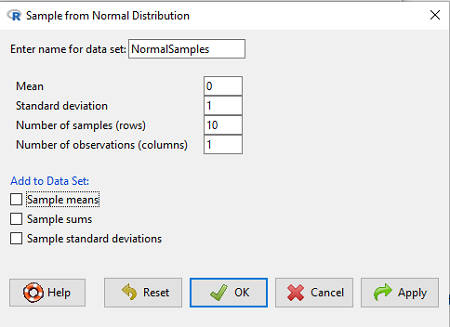
Figure 5. Screenshot Rcmdr menu, sample from a normal distribution.
The menu pops up. I entered Mean (μ) = 0 and Standard deviation (σ) = 1 number of samples = 10, unchecked all boxes under the “add to data set.” I left the object name as “NormalSamples,” you can, of course, change it as needed. R code derived from these requests were
normalityTest(~obs, test="shapiro.test", data=NormalSamples)
NormalSamples <- as.data.frame(matrix(rnorm(10*1, mean=0, sd=1), ncol=1))
rownames(NormalSamples) <- paste("sample", 1:10, sep="")
colnames(NormalSamples) <- "obs"
This results in a new data.frame called NormalSamples with a single variable called obs.
Note 2: About pseudorandom number generator, PRNG. An algorithm is used for creating a sequence of numbers that are like random numbers. We say “like” or “pseudo” random numbers because the algorithm requires a starting number called the seed, rather than a truly random process, ie, a source of entropy outside of the computer. The default PRNG algorithm in base R is Mersenne Twister (Wikipedia), though there are many others included in base R (bring up the help menu by typing ?RNGkind at the prompt), as well as other packages, like random, which can be used to generate truly random numbers (source of entropy is “atmospheric noise,” per citation in the package, see also random.org).
rnorm() was the function used to sample from a normal distribution. If you run the function over and over again (eg, use a for loop), each time you will get different samples. For example, results from three runs
for (i in 1:3){
print(rnorm(5))
}
[1] -0.4221672 -1.4317800 -1.8310352 0.4181184 -1.1596058
[1] -0.2034944 1.1809083 1.5925296 -2.0763677 1.6982357
[1] -1.0967218 -0.3205041 -1.7513838 -0.3335311 -1.8808454
However, if you set the seed to the same number before calling rnorm, you’ll get the same sampled numbers.
for (i in 1:3){
set.seed(1)
print(rnorm(5))
}
[1] -0.6264538 0.1836433 -0.8356286 1.5952808 0.3295078
[1] -0.6264538 0.1836433 -0.8356286 1.5952808 0.3295078
[1] -0.6264538 0.1836433 -0.8356286 1.5952808 0.3295078
The seed number can be any number, it does not have to equal 1.
After creating a sample of numbers drawn from the normal distribution, make a histogram, Rcmdr: Graphs → Histogram… (see Chapter 4.2).
The normal distribution
More on the importance of normal curves in a moment. Sometimes people call these “bell-shaped” curves. You may also see such distributions referred to as Gaussian Distributions, but the normal curve is but one of many Gaussian -type distributions. Moreover, not all “bell-shaped” curves are NORMAL. For a distribution to be “normally distributed” it must follow a specific formula.
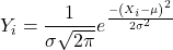
This formula has a lot of parts, but once we break down the parts, we’ll see that there is just two things to know. First, let’s identify the parts of the equation:
 is the height of the curve (normal density)
 (pie) is a constant = 3.14159… (R, use
pi)
µ is the population mean
σ2 is the population variance
σ is the square-root of the variance or the population standard deviation
e is the natural logarithm (R, use exp())
 is the individual’s value
Why the Normal distribution is so important in classical statistics
With these distinctions out of the way, the first important message about the normal curve is that it permits us to say how likely (ie, how probable) is a particular value if the observation comes from a population with mean µ and standard deviation σ and the population from which the sample was drawn came from a normal distribution.
The second message: all we need to know to recreate the normal distribution for a set of data is the mean and the variance (or the standard deviation) for the population!! With just these two parameters, we can then determine the expected proportion of observations expected for each value of X. Note — we generally do not know these two because they are population parameters: we must estimate them from samples, using our sample statistics, and that’s where the first big assumption in conducting statistical analyses comes into play!!
An example for calculating the normal distribution when knowing the mean and variance
µ = 5, σ2 = 10 (thus, the standard deviation, σ = 3.16)
The formula becomes
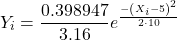
Now, plug in different values of X (for example, what’s the probability that a value of X could be 0, 1, 2, …, 10? If we really do have a normal curve with mean = 5, and variance = 10).
The normal equation returns the proportion of observations in a normal population for each X value:
When i = 5 Y5 = 0.12616 This is the proportion of all data points that have an X = 5 When i = 1 Y1 = 0.019995 This is the proportion of all data points that have an X = 1
We can keep going, getting the proportion expected for each value of X, then make the plot (Fig 6).
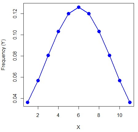
Figure 6. Frequency expected for a few points (X: 0 – 10) drawn from a normal distribution, calculated using the formula and example values.
Here’s the R code for the plot
X = seq(0,10, by=1)
Y = (0.398947/3.16)*exp((-1*(X-5)^2)/20)
plot(Y~X, ylab="Frequency (Y)", cex=1.5, pch=19,col="blue")
lines(X,Y, col="blue", lwd=2)
Next up, more about the normal distribution, Chapter 6.7.
Questions
- For a mean of 0 and standard deviation of 1, apply the equation for the normal curve for X = (-4, -3.5, -3, -2.5, -2, -1.5, -1, -0.5, 0, 0.5, 1, 1.5, 2, 2.5, 3, 3.5, 4). Plot your results.
- Sample from a normal distribution with different sample size, means, and standard deviations, each time make a histogram and compare the shape of the histograms.
- For a subset of
Quiz Chapter 6.6
Continuous distributions
Chapter 6 contents
- Introduction
- Some preliminaries
- Ratios and proportions
- Combinations and permutations
- Types of probability
- Discrete probability distributions
- Continuous distributions
- Normal distribution and the normal deviate
- Moments
- Chi-square distribution
- t distribution
- F distribution
- References and suggested readings