14.6 – Some other ANOVA designs

Introduction
Two-way randomized complete block design
Two-way factorial with no replication design
Repeated measures ANOVA
Three-way ANOVA
ANOVA designs without random assignment to treatment levels
Questions
Quiz
Chapter 14 contents

Introduction

There are several additional ANOVA models in common use. The crossed, balanced design is but one example of the two-way ANOVA. And, from a consideration of two factors it logically follows that there can be more than two factors as part of the design of an experiment. As the number of factors increase, the number of two-way, three-way, and even higher-order interactions are possible and at least in principle may be estimated.

Our purpose here is to highlight several, but certainly not all possible experimental designs from the perspective of ANOVA. Examples are provided. Keep in mind that the general linear model approach unifies these designs.

Some of the classical experimental ANOVA designs one sees include

Two-way randomized complete block design
Two-way factorial with no replication design
Repeat-measures ANOVA with one factor
Nested ANOVA
Three-way ANOVA
Split-plot ANOVA
Latin squares ANOVA

Put simply, these designs differ in how the groups are arranged and how members of the groups are included.

Two-way randomized complete block design

This design refers to the “textbook” design. For each, factor A and factor B, there are multiple levels, in this example three levels of Factor A and three levels of Factor B, and subjects (sampling units) are randomly assigned to each level. However, one of the factors is, perhaps, of less interest, yet certainly accounts for variation in the response variable.

		Factor B
		1	2	3
Factor A	1	$n_{1,1}$	$n_{1,2}$	$n_{1,3}$
	2	$n_{2,1}$	$n_{2,2}$	$n_{2,3}$
	3	$n_{3,1}$	$n_{3,2}$	$n_{3,3}$

where n_1,1, n_2,1, etc. represents the number of subjects in each cell. Thus, in this design there are nine groups. Typically, minimum replication would be three subjects per group.

Two-way factorial with no replication design

While it may seem obvious that a good experiment should have replication, there are situations in which replication is impossible. While this seems rather odd, this scenario very much describes a typical microarray, gene expression project.

		Factor B
		1	2	3
Factor A	1	$n_{1,1}$	$n_{1,2}$	$n_{1,3}$
	2	$n_{2,1}$	$n_{2,2}$	$n_{2,3}$
	3	$n_{3,1}$	$n_{3,2}$	$n_{3,3}$

where, again, n1,1, n2,1, etc., represents the number of subjects in each cell and there are nine groups in this study. With no replication, then no more than one subject per group.

Repeated-measures ANOVA

When subjects in the study are measured multiple times for the dependent variable, this is called a repeated-measures design. We introduced the design for the simple case of before and after measures on the same individuals in Chapter 12.3. It’s straight-forward to extend the design concept to more than two measures on the subjects. The blocking effect is the individual (see Chapter 14.4), and, therefore, a random effect (see Chapters 12.3 and 14.3) in this type of experimental design.

Although straightforward in concept, repeated measure designs have many complications in practice. For example, long-term studies can expect for subjects to drop out of the study, resulting in censored data. Another complication, the assumption is that there is no carry over effect — it doesn’t matter the order different treatments are applied to the subjects. Think of this assumption as akin to the equal variances assumption in ANOVA; just like unequal variances effects Type I error rates in ANOVA, deviations from sphericity inflate Type I error rates in repeated-measures designs.

Sphericity assumption is described in two ways:

Assumption of sphericity — the ranking of individuals remains the same across treatment levels — no interaction between individual and treatment. Sphericity assumption is always met if there are just two levels of the repeated measure, eg, before and after.

Compound symmetry assumption — the variances and covariances are equal across the study: the changes experienced by the subjects are the same across the study regardless of the order of treatments.

Tests for sphericity include:

Mauchly test: mauchly.test(object)

If results of tests for violations of sphericity warrant, corrections are available. One recommended correction is called Greenhouse-Giesser correction, which adjusts the degrees of freedom and so results in a better p-value estimate. A second correction is called Huyhn-Feldt correction; this correction, too, adjusts the degrees of freedom to improve the p-value estimate.

Three-way ANOVA

It is relatively straightforward to imagine an experiment that involves three or more factors. The analysis and interpretation of such designs, while feasible, becomes somewhat complicated especially for the mixed models (Model III).

Consider just the case of a fixed-effects 3-way ANOVA. How many tests of null hypotheses are there?

Three tests for main effects.
Three tests of two-way interactions.
A test for a three-way interaction.

Thus, there are seven separate null hypotheses from a three-way ANOVA with fixed effects! As you can imagine, large sample sizes are needed for such designs, and the “higher-order” interactions (eg, three-way interaction) can be difficult to interpret and may lack biological significance.

ANOVA designs without random assignment to treatment levels

Latin square design

We have introduced you to several ANOVA experimental designs that employed randomization for assignment of subjects to treatment groups. The purpose of randomization is even out differences due to confounding variables. However, if we know in advance something about the direction of the influence of these confounding variables, strictly random assignment is not in fact the best design. For example, the Latin square design is common in agriculture research and is very useful for situations in which two gradients are present (eg, soil moisture levels, soil nutrient levels).

	Dry soil ←→ Wet soil
Soil Nutrients low ↑ ↓ high	T1	T4	T3	T2
	T3	T2	T1	T4
	T2	T3	T4	T1
	T4	T1	T2	T3

Split-Plot Design

Another design from agriculture research is especially useful to ecotoxicology research. We mentioned the repeated measures design in which individuals are measured more than once and each individual receives all levels of the treatment in a random order (cross-over design). However, this design assumes that there are no carry-over effects (see Hills and Armitage 1979; For ecology/evolution definition see O’Connor et al 2014). While this assumption may hold for many experiments, we can also imagine many more situations in which this is undoubtedly false. For example, if we wish to measure the effects of ozone and relative humidity on frog behavior, we might consider using the individual as its own control. But we also wish to compare frog behavior following ozone exposure against behavior exhibited in clean air. But we are likely to violate the carry-over assumption. If a frog receives ozone then air, the effects of ozone may inhibit activity for several days after the initial exposure, which would then influence subsequent measures. The solution to this dilemma is to use what’s called a split plot design. The design combines elements of nesting.

Consider our frog experiment. There would be three factors:

Factor 1 = Exposure (air or ozone),

Factor 2 = Saturation (dry, intermediate, wet),

Factor 3 = Individual (each frog is measured 3 times).

The design table would look like

		Exposure
		Air			Ozone
Humidity	Dry	Frog1	Frog2	Frog3	Frog4	Frog5	Frog6
	Intermediate	Frog1	Frog2	Frog3	Frog4	Frog5	Frog6
	Wet	Frog1	Frog2	Frog3	Frog4	Frog5	Frog6

Thus, the design is crossed for one factor (saturation), but nested for another factor (individuals are nested within Exposure factor).

Questions

Which of the study designs mentioned so far are sensitive to carry-over effects?
With respect to how levels of Factors are assigned, distinguish the split-plot design from the Latin square design.

Quiz Chapter 14.6

Some other ANOVA designs

Chapter 14 contents

5.2 – Experimental units, Sampling units

Introduction
Experimental units
Experimental and sampling units often, but not always the same
Replication: Groups and individuals as sampling units
Conclusion
Questions
Quiz
Chapter 5 contents

Introduction.

Sampling units refer to the measured items, the focus of data collection; samples are selected from populations. Often, sampling units are the same thing as individuals. For example, if we are interested in the knowing whether men are more obese than women in Hawai’i, we would select individuals from the population; we would measure individuals. Thus, the sampling unit would be individuals, and the measurement unit would be percent body fat recorded for each individual. The data set would be the collection of all body fat measures for all individuals in the study, and we would then make inferences (draw conclusions) about the differences, if any, between adult males and females for body fat.

But sampling units can also refer to something more restrictive than the individual. For example, we may be interested in how stable, or consistent, is a person’s body fat over time. If we take a body fat measure once per year over a decade on the same group of adults, then the sampling unit refers to each observation of body fat recorded (once per year, ten times for an individual), and the population we are most likely to be referring to is the collection of all such readings (ten is arbitrary — we could have potentially measured the same individual thousands of times).

In some cases the researcher may wish to compare groups of individuals and not the individuals themselves. For example, a 2001 study sought to see if family structure influenced the metabolic (glycemic) control of children with diabetes (Thompson et al 2001). The researchers compared how well metabolic control was achieved in children of single parents and two-parent families. Thus, the sampling units would be families and not the individual children.

Experimental units.

Experimental units refers to the level at which treatments are independently applied in a study. Often, but not always, treatments are applied directly to individuals and therefore the sampling units and experimental units in these cases would be the same.

Question 1: What is the sampling unit in the following cell experiment?

A technician thaws a cryo tube containing about ½ million A549 cells (Foster et al 1998) and grows the cells in a T-75 culture flask (the 75 corresponds to 75 cm² growing area) in a CO₂ incubator at 37 °C. After the cells reach about 70% confluency, which may represent hundreds of thousands of cells, the technician aliquots 1000 cells into twelve wells of a plate for a total of 12000 cells. To three wells the technician adds a cytokine, to another three wells he adds a cytokine inhibitor, and to another three wells he adds both the cytokine and it’s inhibitor, and to the last three wells he adds DMSO, which was the solvent for both the cytokine and the inhibitor. He then returns the plate to the incubator and 24 hours later extracts all of the cells and performs a multiplex quantitative PCR to determine gene expression of several target genes known to be relevant to cell proliferation.

The described experiment would be an example of a routine, but not trivial procedure the technician would do in the course of working on the project in a molecular biology laboratory.

The choices for numbers provided in the description we may consider for the number of sampling units are:

1000 cells
12,000 cells
½ million cells
3 wells
12 wells
The target genes
None of the above

The correct answer is E, the 12 wells. In experimental design, the experimental/sampling unit is the smallest physical entity to which a specific treatment is independently applied and from which a measurement is taken. Treatments (cytokine, inhibitor, both, or DMSO) are applied to individual wells, and all cells within a single well are harvested and pooled together for a single qPCR measurement.

To find the sampling unit, work backward from the qPCR measurements to find the smallest entity that is independently treated and measured. The target genes are simply the response variables being measured, and individual cells are not independent because all 1,000 cells in a well share the same medium, receive the same treatment, and are pooled together during extraction. While all cells originate from a single thawed cryo tube, that tube represents the shared stock population rather than the sampling unit. Because the technician independently applies treatments to and harvests each of the 12 wells, each well acts as an independent sampling unit, making the correct answer E. 12 wells.

Experimental and sampling units often, but not always the same.

Question 2: What is the experimental unit in the described cell experiment?

1000 cells
12,000 cells
½ million cells
3 wells
12 wells
The target genes
None of the above

The correct answer is E, 12 wells. Noted above, the technician applied treatments to 12 wells. DMSO was added to all wells. There were three treatments, cytokine, inhibitor, and cytokine-inhibitor (Table 1).

In this experiment, the experimental unit and the sampling unit are both 1 well. They would differ under two main circumstances:

Subsampling Within a Well: If the technician applies treatments to the 12 wells but measures individual cells (eg, via single-cell RNA-seq) or splits each well’s extract into multiple qPCR reactions, the experimental unit is 1 well (12 total), while the sampling unit is 1 cell or 1 reaction.
Treating a Larger Group at Once: If the technician places four 3-well plates into four different incubators (eg, varying CO2 levels) and still harvests each well separately, the treatment is applied to the whole plate. Here, the experimental unit is 1 plate (4 total), while the sampling unit remains 1 well (12 total).

How This Connects to Pseudoreplication

When the experimental and sampling units differ, pseudoreplication occurs if you treat the smaller sampling units as independent experimental units in your statistical analysis (Hulbert 1984; Lazic 2010; Lazic et al 2018). For example, if we measured 100 individual cells from each of the 12 wells and ran a statistical test with n = 1,200 instead of accounting for the 12 wells, you would artificially inflate your sample size and risk false-positive results.

Table 1. Translate experiment description to a table to better visualize the design

Wells	Treatment
A1	Cytokine
A2	Cytokine
A3	Cytokine
A4	DMSO
B1	Inhibitor
B2	Inhibitor
B3	Inhibitor
B4	DMSO
C1	Cytokine+Inhibitor
C2	Cytokine+Inhibitor
C4	Cytokine+Inhibitor
C4	DMSO

💡 Mike’s Tips

Use package ggplate to create a simple graphic to visualize a culture plate.

table01.ch05.2 <- data.frame(
     well = c("A1", "A2", "A3", "B1", "B2", "B3", "C1", 
              "C2", "C3", "A4", "B4", "C4", "D4"),
     treatment = c(rep("Cytokine", 3), rep("Inhibitor", 3), 
              rep("Cytokine + Inhibitor", 3), rep("DMSO", 4))
     )
plate_plot(data = table01.ch05.2, 
     position = Well, 
     value = Treatment,
     plate_size = 12,
     plate_type = "round")

which results in this nice plate layout (Fig 1)

Plate layout for Table 1. Plot made with plate_plot() function from R package ggplate.

Figure 1. Plate layout for Table 1. Plot made with plate_plot() function from R package ggplate.

If observations were made, then the same function can display values. Add a column of values to the dataset (eg, “Values”), then add another value = line, eg, value = Values to the R code.

Replication: Groups and individuals as sampling units.

The correct identification of levels at which sampling independence occurs is crucial to successful interpretation of inferential statistics.

Note 2

Replication in Table 1: three cytokine, three cytokine-inhibitor, three with both.

Sampling error rate is evaluated at the level of the sampling units. Technical replication of sampling units allows one to evaluate errors of measurement (eg, instrument noise) (Blainey et al 2014) and other sources of technical sources of noise.

Note 3

Data noise refers to random or irrelevant information that corrupts the “true” signal in a dataset, introducing variability and potential errors. A nuisance variable is a specific type of noise that is fundamental to the data collection process but not of interest to the researcher, and its effect must be accounted for or removed via pre-processing steps. For approaches to control for noise, see Chapter 17.4 and Chapter 20.3 for more.

Replication of sampling units increases statistical power, the ability to correctly reject hypotheses. If the correct design reflects sampling units are groups and not individuals, then by counting the individuals as the independent sampling units would lead the researcher to think his design has more replication than it actually does. The consequence on the inferential statistics is that he will more likely reject a correct null hypothesis, in other words, the risk of elevated type I error occurs (Chapter 8 – Inferential statistics). This error, confusing individual and group sampling units, is called pseudoreplication (Lazic 2010).

Consider a simpler experimental design scenario depicted in Figure 2: Three different water treatments (eg, concentrations of synthetic progestins, Zeilinger et al. 2009) in bowls A, B, and C; three fish in bowl A, three fish in bowl B, and three fish in bowl C. The outcome variable might be a stress indicator, eg, plasma cortisol (Luz et al 2008).

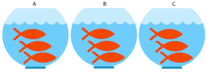
Figure 2. Three aquariums, 3 fish. Image modified from https://www.pngrepo.com/svg/153528/aquarium

Figure 2. Three aquariums, three fish. Image modified from https://www.pngrepo.com/svg/153528/aquarium

Question 3: What were the experimental units for the fish in the bowl experiment (Fig 2)?

Three bowls
Nine fish
Three water treatments

The correct answer is A, 3 bowls. The treatments were allocated to the bowls, not to individual fish. The three fish in each bowl provides technical replication for the effects of bowl A, bowl B, and bowl C, but does not provide replication for the effects of the water treatments. Adding three bowls for each water treatment, each with three fish, would be the simplest correction of the design, but may not be available to the researcher because of space or cost limitations. The design would then include nine bowls and 27 fish. If resources are not available to simply scale up the design, then the researcher could repeat the study several times, taking care to control nuisance variables (Chapter 5.3). Alternatively, if the treatments were applied to the individual fish, then the experimental units become the individual fish and the bowls reduced to a blocking effect (Chapter 14.4), where differences may exist among the bowls, but they are no longer the level by which measurements are made.

Note 4

If pseudoreplication is present in a study, then this may be accounted for by specifying the error structure in a linear mixed model (eg, random effects, blocking effects, etc., see Chapter 14 and Chapter 18).

Question 4: What were the sampling units for the fish in the bowl experiment (Fig 2)?

Three bowls
Nine fish
Three water treatments

The correct answer is B, the individual fish. If instead of aqueous application of synthetic progestin, treatments were applied directly to each fish via injection, what would be the answers to Question 3 and Question 4?

Choices like these clearly involve additional compromises and assumptions about experimental design and inference about hypotheses.

Conclusion.

Sampling units, experimental units, and the concept of level at which units are independent within an experiment were introduced. Lack of independence yields the problem of pseudoreplication in an experiment, which will increase the chance that we will detect differences between our treatment groups, when no such difference exists!

Questions.

Figure 3. Three Miracle-Grow AeroGarden planters, each with nine seedlings of an Arabidopsis thaliana strain.

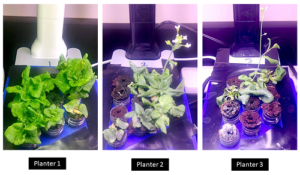
Figure 3. Three Miracle-Gro AeroGarden planters®, each with nine seedlings of an Arabidopsis thaliana strain.

Nine seeds each of three strains of Arabidopsis thaliana were germinated in three Miracle-Grow AeroGarden^® hydroponic planters (Fig 3). Each planter had nine or ten vials with sphagnum peat. All seeds from a strain were planted in the same apparatus, one seed per vial. With respect to this experimental design

1. Define experimental units and sampling units.

2. Provide design examples where the experimental units are the same as the sampling units.

3. With respect to the independent and dependent (outcome) variables, discuss impacts of nuisance variables.

Quiz Chapter 5.2

Experimental units, Sampling units

Chapter 5 contents

The basics explained
Experiments
Experimental and Sampling units
Replication, Bias, and Nuisance Variables
Clinical trials
Importance of randomization in experimental design
Sampling from Populations
References and suggested readings