14.8 – More on the linear model in Rcmdr
Introduction
During the last lectures, we could have used the Two-Way ANOVA command in R or Rcmdr
R code: How to analyze multifactorial ANOVA problems
Rcmdr: Statistics → Means → Multiway ANOVA
To analyze our two factor data sets. As long as the design meets the following conditions, by all means use this command because it is simple and precisely correct.
- Both factors are fixed, not random.
- Each level of first factor is crossed with each level of the second factor.
- No missing data (the design is fully replicated and balanced).
If any of the three points do not fit your two-way design, then you’ll need a different, more general and powerful ANOVA procedure in R and Rcmdr to analyze these types of designs. You’ll need the lm() function (Fig 1).
Rcmdr: Statistics → Fit models → Linear model…
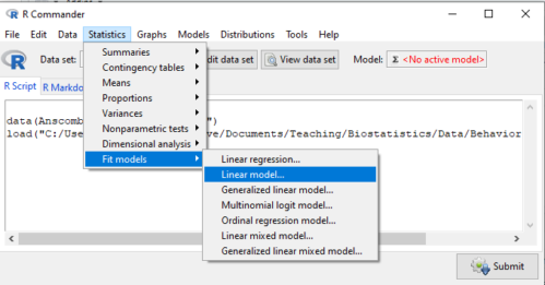
Figure 1. Linear model menu in Rcmdr, version 2.7.0
Some R basics with the lm() function, the general linear model.

Response  is specified by linear predictor(s), either factors or covariates (ratio-scale predictor variables). We communicate to R what the model is by using operators. The four more commonly used operators are
 the basic way to include the model terms, ie, the mode predictors
 which is interpreted as the interaction of all the variables and the factors in the term
 is interpreted as factor crossing
Not shown, but  indicates the term on the left is nested within the term on the right.
A few examples: we’ll have three factors, A, B, and C. For our one-way ANOVA, the model specification would be

For our crossed, balanced two-way ANOVA, the model specification would be

or equivalently

And for our block ANOVA problem?
Click here to get entire List of model commands in R.
How would we analyze our snake experiment?
Table 1. The snake data set
| Snake | Source | flick |
| 1 | dH2O | 3 |
| 2 | dH2O | 0 |
| 3 | dH2O | 0 |
| 4 | dH2O | 5 |
| 5 | dH2O | 1 |
| 6 | dH2O | 2 |
| 1 | fish | 6 |
| 2 | fish | 22 |
| 3 | fish | 12 |
| 4 | fish | 24 |
| 5 | fish | 16 |
| 6 | fish | 16 |
| 1 | worm | 6 |
| 2 | worm | 22 |
| 3 | worm | 12 |
| 4 | worm | 24 |
| 5 | worm | 16 |
| 6 | worm | 16 |
We have two factors, but one factor is a Block (repeated measures on individuals). We need to tell R and Rcmdr what our model is. We’ll return to talk about models next time, a very important topic!! For now, think of a model as adding the independent variables together to predict the response variable.
In our Snake example, it’s a two-way ANOVA, but one factor is individual snake, the other is a treatment, and we have repeat measures, so there cannot be an interaction.
We tell R and Rcmdr which columns contain the Response, and under Model, we enter the columns with the two factors.
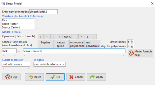
Figure 2. Menu of linear model with repeat measures model, Rcmdr, version 2.7.0.
You must also tell R and Rcmdr which factors in the model (if any) are random to get the correct F statistics. Almost without exception, blocking factors are always treated as Random
The output looks like this (see below). More complicated, true (which means more information!), but things marked in red we’ve seen before.
LinearModel.2 <- lm(flick ~ Snake +Source, data=L16SnakeTaste)

summary(LinearModel.2)

Call:
lm(formula = flick ~ Snake + Source, data = L16SnakeTaste)

Residuals:
Min 1Q Median 3Q Max
-5.2222 -0.7222 0.0278 1.5694 7.4444

Coefficients:
             Estimate Std. Error t value Pr(>|t|)
(Intercept)    -4.444      2.523  -1.762 0.10862
Snake[T.2]      9.667      3.090   3.128 0.01072 *
Snake[T.3]      3.000      3.090   0.971 0.35451
Snake[T.4]     12.667      3.090   4.099 0.00215 **
Snake[T.5]      6.000      3.090   1.942 0.08085 .
Snake[T.6]      6.333      3.090   2.050 0.06755 .
Source[T.fish] 14.167      2.185   6.484 0.0000704 ***
Source[T.worm] 14.167      2.185   6.484 0.0000704 ***
---
Signif. codes: 0 '***' 0.001 '**' 0.01 '*' 0.05 '.' 0.1 ' ' 1

Residual standard error: 3.784 on 10 degrees of freedom
Multiple R-squared: 0.8858, Adjusted R-squared: 0.8058
F-statistic: 11.08 on 7 and 10 DF, p-value: 0.0005337
Contrast coding
When a factor (categorical variable) is used in a linear model (lm() or aov()), R must convert the factor into one or more numeric predictor variables. Contrast coding tells us how to represent the factor in the model, how to interpret the coefficients associated with the factor, how the hypothesis tests of the coefficients are handled, and whether or not Type III sums of squares tests are valid. R can handle contrast coding in a couple of ways, either as a dummy contrast (each group if the factor is contrasted to a baseline) or effects coding, where group means are compared to the grand mean. The command summary(lm()) reports contrast coding that was used in the linear model. Every kind of contrast leads to the same fitted values and same overall F-test, but coefficient estimates and t-tests change.
Note 1: Type I sums of squares tests are affected by the order of the predictors in the model, not by type of contrast coding used. R Commander defaults to Type II tests, which are generally unaffected by coding contrasts used. In contrast, Type III tests are affected by the type of coding contrasts used — Type III tests require sum-to-zero (effects) contrasts.
For the ANOVA table, we call up the command via
Rcmdr: Models → Hypothesis tests → ANOVA table… (Fig 3).
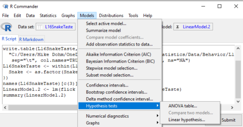
Figure 3. Rcmdr: Models → Hypothesis tests → ANOVA table… Rcmdr, version 2.7.0
Confirm that the model object is active (in this case, the object was LinearModel.2), accept the defaults about types of tests and marginality, and submit OK. The output is
Anova(LinearModel.2, type="II")
Anova Table (Type II tests)

Response: flick
          Sum Sq Df F value Pr(>F)
Snake     307.61  5  4.2956 0.02396 *
Source    802.78  2 28.0256 0.00007954 ***
Residuals 143.22 10
---
Signif. codes: 0 '***' 0.001 '**' 0.01 '*' 0.05 '.' 0.1 ' ' 1
End R output
You do not need to know all of the output; all of that output is there for a reason, of course, but for now, here’s what R and Rcmdr has to say (from the help menu):
The sequential sums of squares is the added sums of squares given that prior terms are in the model. These values depend upon the model order. The adjusted sums of squares are the sums of squares given that all other terms are in the model. These values do not depend upon the model order.
You should try our snake example again, but this time, remove the tongue flick response to the dH2O for the first snake — a missing value. (just type into the cell NA).
How would you use GLM to analyze a simple two-way ANOVA, a fully crossed, fully replicated (“balanced”) design? We could use the Two-way ANOVA command in R and Rcmdr, or we could use lm(). Try it with the data set from random vs nonrandom lecture.
Another example
Below, you see how the model is entered. To let R know that I wish R and Rcmdr to test the interaction, I need to add a Model term for that source of variation. I accomplish this by typing “Diet*Drug” (without the quotes).

Figure 4. Crossed, balanced design. Linear model menu, Rcmdr, version 1.9.2
After clicking OK, the following output from the lm function is returned. How does this compare to output from the two-way ANOVA command in R and Rcmdr?
You should try both and compare!
Rcmdr: Models → Hypothesis tests → ANOVA table
Anova(LinearModel.17, type="II")
Anova Table (Type II tests)
Response: chol_randomized
             Sum Sq  Df F value   Pr(>F)
diet         141.08   2  1.3061 0.28745
drug         351.88   2  3.2577 0.05403 .
diet:drug    235.50   4  1.0901 0.38124
Residuals   1458.19  27
End R output
Nested ANOVA
The nested ANOVA may be analyzed in multiple ways in R and Rcmdr, but I prefer the lm() function because it is the most general. For Nested ANOVA, we can also use lm(). Here’s where it gets a little tricky. Put in the Response variable (Chol), then click in the box for model: Select both factors, then type in / after the factor that’s nesting factor. For our nested model example (14.5 – Nested designs), Manufacturer Source was nested within Drug.
Table 3. Nested design example data set from Chapter 14 – Nested design
| Drug | Source | Chol |
| 1 | 1 | 202.6 |
| 1 | 1 | 207.8 |
| 1 | 1 | 190.2 |
| 1 | 1 | 211.7 |
| 1 | 1 | 201.5 |
| 1 | 2 | 189.3 |
| 1 | 2 | 198.5 |
| 1 | 2 | 208.4 |
| 1 | 2 | 205.3 |
| 1 | 2 | 210 |
| 2 | 3 | 212.3 |
| 2 | 3 | 204.4 |
| 2 | 3 | 221.6 |
| 2 | 3 | 209.2 |
| 2 | 3 | 222.1 |
| 2 | 4 | 203.6 |
| 2 | 4 | 209.8 |
| 2 | 4 | 204.1 |
| 2 | 4 | 201.8 |
| 2 | 4 | 202.6 |
| 3 | 5 | 189.1 |
| 3 | 5 | 219.9 |
| 3 | 5 | 196 |
| 3 | 5 | 205.3 |
| 3 | 5 | 204 |
| 3 | 6 | 194.7 |
| 3 | 6 | 192.8 |
| 3 | 6 | 226.5 |
| 3 | 6 | 200.9 |
| 3 | 6 | 219.7 |
Note 2: If you were working with a CROSSED model, then you would enter the two factors and indicate the interaction by typing Drug*Source (if these are the two factors involved in the interaction).
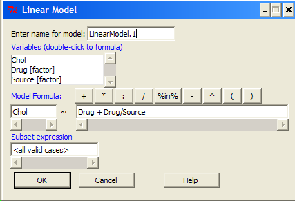
Figure 5. Nested design, linear model menu, Rcmdr, version 1.9.2
Fortunately, R and Rcmdr’s help system is quite extensive here, so when in doubt, check the help box…
Output from the linear model for the Nested Example looks like the one below.
The General Linear Model function in R and therefore Rcmdr returns information about our design plus Sums of Squares, Mean squares, and P-values. R and Rcmdr default’s to use of sequential evaluation of effects. Adjusted evaluation is useful for when you have a covariate (like body size or another confounding variable) that should be evaluated first before the factors are evaluated. We will use the sequential analysis.
Rcmdr: Models → Hypothesis tests → ANOVA table
Anova(LinearModel.15, type="II")
Anova Table (Type II tests)
Response: Chol
             Sum Sq Df F value Pr(>F)
Drug         225.14  2  1.1743 0.3262
Drug:Source  269.27  3  0.9363 0.4385
Residuals   2300.61 24
End R output
Repeatability and ANOVA
We need to tell Rcmdr how to structure the error term; you need the data frame to be arranged so
aovRes <- aov(dH2O ~ Source + Error(Source/Subject), data=SnakeTaste)
#Print the results
aovRes
Anova Table (Type II tests)
Response: dH2O
            Sum Sq Df F value   Pr(>F)
Subject     307.61  5  4.2956 0.02396 *
Source      802.78  2 28.0256 0.00007954 ***
Residuals   143.22 10
---
Signif. codes:  0 '***' 0.001 '**' 0.01 '*' 0.05 '.' 0.1 ' ' 1
#What components are available in the aovRes object?
names(aovRes)
[1] "Sum Sq"  "Df"      "F value" "Pr(>F)"
How do I extract the “F value” for Subjects?
str(aovRes)
Questions
1. What are three learning objectives from this page?
2. Be able to distinguish use of lm() and aov() and the summary output with respect to testing of linear models.
Quiz Chapter 14.8
More on the linear model in Rcmdr
Data sets
Table 1. The snake data set
| Snake | Source | flick |
| 1 | dH2O | 3 |
| 2 | dH2O | 0 |
| 3 | dH2O | 0 |
| 4 | dH2O | 5 |
| 5 | dH2O | 1 |
| 6 | dH2O | 2 |
| 1 | fish | 6 |
| 2 | fish | 22 |
| 3 | fish | 12 |
| 4 | fish | 24 |
| 5 | fish | 16 |
| 6 | fish | 16 |
| 1 | worm | 6 |
| 2 | worm | 22 |
| 3 | worm | 12 |
| 4 | worm | 24 |
| 5 | worm | 16 |
| 6 | worm | 16 |
Chapter 14 contents
5.3 – Replication, Bias, and Nuisance Variables
Introduction
This page describes additional elements of experimental design, replication and bias, which can impact the validity of a study.
Replication in science refers to repeating an experiment under identical conditions multiple times. To the extent the same conclusions are achieved, we can say the outcome is reproducible (Simmons 2014) and, therefore, likely to be objectively true (Earp 2011). Replication of experimental and sampling units is an essential component of good experimental design. Confusing technical replicates for biological replicates is called pseudoreplication.
Bias refers to any of a number of sociological and cognitive errors which may influence conclusions in science (Ionnidis 2005). In a meta-analysis, Fanelli et al (2017) reported that while the size of effect from identifiable biases were small, some disciplines were more prone to these sources of error. That researchers testing similar hypotheses reach different conclusions may result from bias. One such bias is positive outcome bias, where reports of null hypotheses are more often rejected than they should be based on sample size and other concerns of statistical power (see Chapter 11 – Power analysis).
The page concludes with a discussion of nuisance variables, variables that may be causally associated with the outcome of interest, but themselves are either of no interest in the study, or may not be known in advance (Meehl 1970; see also discussion of spurious correlations in Chapter 16.3 – Data aggregation and correlation).
Technical vs. biological replicates.
A laboratory technician retrieves a vial of an immortalized cell line from cryostorage and initiate propagation of the cells for the week’s work. After a couple of days of subculturing, the technician has grown millions of cells and is ready to set up an assay. After washing the cells in PBS (phosphate buffered saline), the technician adjusts the concentration of cells to 10,000 per mL media, places the tube on ice, and proceeds to set up a 48 well microplate. To each well, the technician adds media, one or more agents (Table 1), plus cells, total volume each well at one mL, three replicates per treatment.
Table 1. In our example there were four treatments plus a control (media only)
- DMSO only (D)
- DMSO + Cytokine (DC)
- DMSO + Small molecule Inhibitor (DS)
- DMSO + Cytokine + Small molecule Inhibitor (DCS)
- Media only (M)
The plate table might look something like Figure 1.

Figure 1. Schematics of a set up for a hypothetical 48 well microplate (plate_plot() from ggplate package).
The technician has done a lot of work; but, from a statistician’s point of view, effectively the technician has but one sampling unit to show for his efforts; one biological sampling unit because as far as we can tell, the cells were all related. Biological replication refers to repeat measures (eg, same conditions) on biologically distinct entities (Blainey et al 2014). Technical replication, in contrast, refers to repeat measures on the same entity, eg, the same individual (Blainey et al 2014).
However, there were more than one technical samples in the experimental design, twelve in all because there were twelve wells. Many of you will recognize this as the distinction between technical and biological replicates. In thinking about experimental design replicates pertain to the number of sampling units that are treated the same way. In our example cells may be “treated the same way” in at least two distinct ways. Biologically, the cells may be the same: derived from the same clonal cell, all at the same passage (generation) number, each cell genetically, morphologically, physiologically (etc.,) identical to the next cell. Technical replication on the other hand pertains to the levels of the treatments.
Within each of these treatments we had three wells, and that’s at the level of the technical replication.
A final note on this experiment. We as molecular biologists call each of these treatment groups, but statisticians thinking of this design would recognize only one treatment (called in statistics a factor), with four levels of the treatment. We will discuss this beginning in chapter 12 when we introduce analysis of variance.
Types of bias.
When we make decisions, we like to think we are rational; that we make decisions based on an evaluation of evidence. And yet, an increasing body of literature suggests that our decisions often made in a manner that falls short of rational processing. We outlined some sources of bias in Chapter 2.6. Deviance from rational decision making is due to any number of cognitive biases we may have. Researchers and medical doctors make many decisions and, unfortunately, are just as susceptible to cognitive biases as the rest of us. One kind of bias that is bedeviling to research is confirmatory bias. Confirmatory bias refers to a researcher in effect seeking evidence in a way that confirms a prior conclusion (Kaptchuck 2003). Confirmatory bias would be exhibited if we report positive effects of aspirin to relieve migraines in subjects, but exclude cases where the subjects report no improvement. Medical doctors may be risk averse and therefore tend to over-prescribe, or they may be risk-takers (eg, rise and fall of high-dose chemotherapy, cf, discussion in Howard et al. 2011).
The concept of bias was first introduced in Chapter 3 and will be returned to in subsequent chapters. In general, bias refers to the objectivity of measurement and inferences about such measurements. Bias implies that a series of measurements consistently fail to return the true value of the variable. Bias is systematic error and may be associated with a poorly calibrated instrument or even the use of improper sets of rules for measurement given the nature of the characteristic. Bias can be captured by the concept of accuracy.
Bias is challenging to eliminate; the best way is to design the experiment so that the observer, the researcher, is unaware of the specific questions to be tested. The research is conducted “blind.” Clinical research provides the easiest examples. A trial can be blind in a couple of ways:
- The subjects do not know which treatment they receive, but the researcher does know
- The researcher does not know which treatment subjects receive, but the subjects know
- Neither the researcher nor the subjects know which treatment they receive.
- The other possibility is that both the researcher and the subjects know treatments received — this would be a poor design.
Bias can enter a research project at multiple levels. A partial list of sources of bias in research includes (modified after Pannucci and Wikins 2010):
Bias that occurs before the experiment
- Inadequate planning of the experiment, flawed design
- Bias in selection of subjects from the reference population
- Surveillance bias, where one group is studied more closely than another group.
Surveillance bias, also called detection bias or ascertainment bias, a type of information bias. Characterized as “the more you look, the more you find (Sackett 1979),” differences in outcome counts varies with differences in effort to detect. Recently, cases of myocarditis in young people were reported following Covid-19 mRNA vaccination (eg, Bozkurt et al 2021. Marshall et al 2021). However, myocarditis reports following vaccination occur at the rates expected in the population, and the reports lack important context (eg, other respiratory viruses known to cause myocarditis not ruled out), suggesting the putative link between Covid-19 vaccines and this heart condition may be result of us looking hard for signs of adverse effects of the vaccine (cf, discussion in O’Leary and Maldonado 2021).
Bias during the experiment
- Interviewer bias
- Chronology bias
- Recall bias
- Transfer bias
- Misclassification of exposure or outcome
- Performance bias
Performance bias refers to conditions of an experiment that introduce unintended differences between groups. For example, subjects enrolled in a weight-loss study randomly assigned to the control group may react poorly when they realize they are not receiving the experimental intervention. This leads to potential for a systematic bias — participants in the control group may behave differently, counteracting the point of randomization (McCambridge et al 2014).
Another well-known performance bias is associated with eliciting maximal performance from animals, such as running stamina or maximum sprint running speed (Losos et al 2002). For example, spring running speed of lizards may be measured by placing lizards onto a high-speed treadmill, then increasing belt speed to match the individual’s burst performance (eg, Dohm et al 1998). Clearly, not all individuals will perform to maximum physiological capabilities under these conditions.
Bias after the experiment
- Citation bias
- Confounding
Another way to view sources of bias is that, at least from the perspective of the researcher, the bias is likely to be unconscious bias. After all, if we knew about the sources of bias we would work our experiments in such a way to minimize known error producing sources (Holman et al 2015). Selecting subjects at random and keeping record keeping blind with respect to treatments are among the best tools we have to avoid this kind of bias.
Nuisance variables
A key quality of experimental design is the opportunity afforded the researcher to apply control. In a classic view of the experiment, one allows only one aspect to vary, the treatment applied, all else is controlled. Thus, any difference in outcome may be attributed to the treatment. However, it is likely impossible to control for all possible variables that may affect our outcome; confounding clear interpretation of results (see Chapter 16.2 and 16.3). Consider, for example, the effects of age on running performance (Fig. 2).
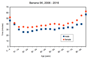
Figure 2. Mean 5K running times (minutes) by age and gender (2006 – 2016, Jamba Juice Banana 5K race, Honolulu, HI).
If we are interested in gender differences, we must also deal with the change in performance with age: older runners regardless of gender tend to run slower than younger runners. Thus, in the comparison of genders, age is a nuisance variable. In the literature, you may see “lurking variable,” or other such names. The concept is that these variables may be causal, but are either of no interest in the study, or may not be known in advance. Therefore, age must be accounted for before we can address gender differences, if any. Age, in this case, is considered a nuisance variable because we are not primarily interested in age effects, but age clearly covaries (is associated) with running performance. How best to handle nuisance variables? One approach is to match by age (blocking effect, see Chapter 14.4); another approach would be to randomly select with respect to age when compiling female and male times.
Another example of confounding. Results from ecological experiments intended to test for presence of competition for resources by plant species by removing plants may alter herbivory levels; thus, survivorship not the result of reduced plant-plant competition but because of changes in herbivore behavior (Reader 1992).
Questions
- I cite a number of articles in Mike’s Biostatistics Book. If you’re paying attention, you’ll have noticed that all of my citations, at least for articles, link to a source that you can either download or read online. What kind of error am I committing by following this approach?
- In large part because of the tendency for overuse of antibiotics, doctors are less likely today to prescribe antibiotics for patients with upper respiratory tract infections than in the past (Zoorob et al 2012). URTI are mostly caused by rhinovirus infections (Calderaro et al 2022) and, therefore, the course of infection in a patient should be unaffected by addition of antibiotic. However, although rare compared to URTI, life-threatening illness like acute epiglottitis caused by bacteria infection can sometimes develop or accompany URTI. Thus, not prescribing antibiotics at a diagnosis of URTI may risk a worsening condition for the patients. This sets the doctor up for a potential cognitive bias – to prescribe or not to prescribe antibiotics prophylactically? Discuss this decision in the context of potential sources of cognitive biases and possible outcomes of the decision.
Quiz Chapter 5.3
Replication, bias, and nuisance variables
Chapter 5 contents
- The basics explained
- Experiments
- Experimental and Sampling units
- Replication, Bias, and Nuisance Variables
- Clinical trials
- Importance of randomization in experimental design
- Sampling from Populations
- References and suggested readings