3.4 – Estimating parameters
Introduction.
What you will find on this page. Definitions for constants, variables, and parameters as used in data analytics. Statistical bias and the concept of unbiased estimators are discussed. The different types of error are introduced along with definitions of accuracy and precision. Statistics used to quantify error are presented in the next section, Chapter 3.4.
Estimating parameters.
Parameters belong to populations; they are fixed but unknown. Parameters are characteristics of populations: the typical average height and weight of five year old children; What is the normal range of values for height and weight of five year old children; average and range of gene expression of TP53 in epithelial lung cells of 50 year old non-smoking humans; etc. Because we generally do not have at our disposal surveys — census — of entire populations for these characteristics, we sample and calculate descriptive statistics for a subset of individuals from populations: these statistics, the mean height, range of height, etc., are variables. We expect average height, range of height, etc., to change, to vary, from sample to sample. A constant, as the word implies, is not variable and remains unchanged.
We estimate parameters (means, variances) from samples of observations from a population. Intuitively then, our estimates are only as good as how representative of the population the sample is. Statistics allows us to be more precise: we can define “how good” our estimates are by asking about, and quantifying, the accuracy and precision of our estimates.
Notwithstanding the notion of “personalized medicine,” our goal in science is to understand cause and effect among sets of observations on samples from a population. We ask, what is the link between lung cancer and smoking? We know that smoking tobacco cigarettes increases risk of cancer, but not everyone who smokes will get cancer (Pesch et al., 2012). Tumorigenic risk is in part mediated by heredity (cf. Trifiletti et al 2017). That’s one way we run into problems in statistics: the biological phenomenon is complicated in ways we are not yet aware of, and thus samples drawn from populations are heterogeneous. Put another way, we think there is one population, but there may be many distinct populations. By chance, repeated samples drawn from the population include individuals with different risk associated with heredity.
As an aside, this is precisely why the concept of personalized medicine is important. Medical researchers have learned that some people with breast cancer respond to treatment with trastuzumab, a monoclonal antibody, but others do not (review in Valabrega et al 2007). Responders have more copies of a gene, copy number variation, for an EGF-like receptor called HER2. In contrast, non-responders to trastuzumab have fewer copies of this receptor (and are said to be HER2-negative in an antibody test for HER2). Thus, we speak about people with breast cancer as if the disease is the same, and from a statistical point of view, we would assume that individuals with breast cancer are of the same population. But they are not — and so the treatment fails for some, but works for others. In this example, we have a mechanism or cause to explain why some do not respond; their breast cancer is not associated with increased copy numbers of HER2. And so in studies with breast cancer, statisticians may account for differences in HER2 status. Note: Fewer than 30% of breast cancer may have over-expression of HER2, (Bilous et al. 2003).
Clearly, HER2 status would be used by statisticians when drawing samples from population, and we would not mistake samples. But, in many other situations we are not aware of any differences and so we assume our samples come from the same population. Note that even with imperfect knowledge about samples, experimental design is intended to help mediate heterogeneous samples. For example, this is why treatment controls need to be used, or case controls are included in studies.
Random assignment to groups also is an attempt to control for unknowns: if random, then all treatment groups will likely include representatives of the numerous co-factors that contribute to risk.
Statisticians have an additional, technical burden: there are often a variety of ways (algorithms) to describe or make inferences about samples, and they are not equally capable of giving us “truth.” Estimates of a parameter are not going to be exactly the true value of the parameter! This is the problem of identifying unbiased ways to estimate parameters. In statistics, bias quantifies whether an algorithm to calculate a particular statistic (e.g., the mean or variance), is consistently too low or too high.
Random sampling.
Random sampling from the population is likely to be our best procedure for obtaining representative samples, but it is not foolproof (we’ll return to situations where random sampling fails to provide adequate samples of populations in Chapter 5.5 Importance of randomization in experimental design). However, a second concern is how to calculate the mean, how to calculate the variance. In the section on Descriptive Statistics (Chapter 3.2), we presented how to calculate the arithmetic mean — the simple average — but also introduced you to other calculations for the middle (e.g., median, geometric mean, harmonic mean). How to know which “middle” is correct?
Statisticians use the concept of bias — the simple arithmetic mean is an unbiased estimator of the population parameter, but a correction needs to be made to the calculation of sample variance to remove bias. Bias implies that the estimator systematically misses the target in some way. Good or “best” parameter estimates are, on average, going to be close to the actual parameter if we collected many samples of the population (this will depend on the sample size and the variability of the data). Earlier we introduced Bessel’s correction to the sample variance, divide the sum of squares by n – 1 and not N as we did for the population variance, so that it is an unbiased estimator of the sample variance. Thus, statisticians have worked out how well their statistical equations work as estimators; concepts of expected values or the expectation are used to evaluate how well an estimator works. In statistics, the expected value of a statistic is calculated by multiplying each of the possible outcomes by the likelihood each outcome will occur and then summing all of those values..
We need to add a bit more to our discussion about measurement and estimation.
Types of error.
To measure is to assign a number to something, a variable. Measurements can have multiple levels, but are of the four data types: nominal, ordinal, interval scale, and ratio scale. Nominal and ordinal types are categorical or qualitative; interval and ratio are continuous or quantitative. Errors in measurement represent differences between what is observed and recorded compared with the true value, i.e., the actual population value. With respect to measurement we distinguish between random errors and systematic errors. Random errors occur by chance, and are thus expected to vary from one measurement instance from another. Random error may lead to measures larger or smaller than the true value. Systematic errors are of a kind that can be attributed to failures of an experimental design or instrument.
Accuracy is reflected in the question: how close to the true value is our measure? Accuracy is distinct from precision, the concept of how clustered together are repeated values for the same measurement. All measurement has associated error, which may be divided into two kinds: random error and systematic error.
We tend to think of error in terms of mistakes, mistakes by us or as failure of the measurement process. However, in biology research, that is too restrictive of a meaning for error. First, experimental error occurs when the estimates derived from the samples — sample mean, sample variance — differ from the population parameters — population mean, population variance. Second, error in biology ranges from mistakes in data collection to real differences among individuals for a characteristic. The latter source, error among individuals, is of course, not a mistake, but rather, it’s the “very spice of life” (Cowper 1845). We’ll leave the study of individual differences, biological error, for later. This section is concerned with error in the sense of mistakes.
Random error includes things like chance error in an instrument leading to different repeat measures of the same thing and to the reality that individual differences exist for most biological traits. We minimize the effects of this kind of error by randomizing: we randomly select samples from populations; we randomly assign samples to treatment groups. Random error can make it hard to differentiate treatment effects. Random error decreases precision, the repeatability of measures. At worse, random error is conservative — it tends to mean we miss group differences, we conclude that the treatment (e.g., aspirin analgesics) has no effect on the condition (e.g., migraines). This kind of error is referred to as a Type II error (Chapter 8).
The experimental design remedy for random error is to increase sample size, a key conclusion drawn from power analysis on experiments, discussed in Chapter 11. The other type of error, systematic error, a type of bias, is more in line with the idea of errors being synonymous with mistakes. Uncalibrated instruments yield incorrect measures. And these kinds of errors lead us to make errors that can be more problematic. An example? Back in the early 1990s when I started research on whole animal metabolic rates (e.g., Dohm et al 1994, Beck et al 1995), we routinely set baseline carbon dioxide, CO2, levels to 0.035% of volume of dry air (350 ppm, parts per million), which reflected ambient levels of CO2 at the time (see Figure 4 in Chapter 4.6).
#NOAA monthly data from Mauna Loa Observatory
co2.1994 <- c(358.22, 358.98, 359.91, 361.32, 361.68, 360.80, 359.39, 357.42, 355.63, 356.09, 357.56, 358.87)
You are probably aware, today, background CO2 have increased considerably even since the 1980s. Data for 2021 (average 420 ppm — reporting just 2 significant figures) are provided below
co2.2021 <- c(415.49, 416.72, 417.61, 419.01, 419.09, 418.93, 416.9, 414.42, 413.26, 413.9, 414.97, 416.67)
source: Global Monitoring Lab, NOAA
Thus, if I naively compared rates of CO2 produced by an animal at rest,  , measured today against the data I gathered back in the 1990s without account for the change in background CO2 in my analysis, I will have committed a systematic error: values of on animals would be systematically higher than values for 1988 when I apply a baseline correction.
Examples of error.
One under-reported cost of next-generation sequencing technologies is that base calls, the process of assigning a nucleotide base to chromatogram peaks has more errors than traditional Sanger-based sequencing methods (Fox et al 2014). In “next-generation-sequencing” (NGS) methods, individual DNA fragments are assigned sequences, whereas Sanger methods took the average sequence of a collection of DNA fragments; thus, in principle, NGS methods should be able to characterize variation of mixtures of sequences in ways not available to traditional sequencing approaches. However, artifacts introduced in sample preparation and PCR amplification lead to base calling errors (Fox et al 2014).
Gene expression levels will differ among tissue types, thus mixed samples from different tissues will misrepresent gene expression levels.
Measurement of energy expenditure, oxygen uptake and carbon dioxide release by an organism, have long been sources of study in ecology and other disciplines. A classic measure is called basal metabolic rate, measured as the rate of oxygen consumption of an endothermic animal, post-absorptive (i.e., not digesting food), at rest but not sleeping, while the animal is contained within a thermal-neutral environment (Blaxter 1989).
Accuracy and precision.
Two properties of measurement are the accuracy of the measure and its precision. Accuracy is defined as the closeness of a measured value to its true value. Precision refers to the closeness of a second measure to the first, to the closeness of a third measure to the first and second, and so on. Precision refers to repeatability of measurement. We suggested use of the coefficient of variation, defined with examples in Chapter 3.2, as a way to quantify precision.
Consider the accuracy and precision of three volumetric pipettors: p1000, which has a nominal range between 100 and 1000 μL (microliters); p200, which has a range between 20 and 200 μL; p100, which has a range between 10 and 100 μL. Which of these three pipettors do you think would have the best accuracy and precision for dispensing 100 μL? We can test pipettors by measuring the mass of distilled water dispensed by the pipettor on an analytical balance. For 100 μL of distilled water at standard temperature and pressure conditions, the mass of the water would be 0.100 grams. The results are shown in the table, and a dot plot is shown in the figure to help us see the numbers.
Table 1. Mass (grams) of 100 μL of distilled water dispensed by three volumetric pipettors*
| p1000 | p200 | p100 | |
| 0.113 | 0.100 | 0.101 | |
| 0.114 | 0.100 | 0.100 | |
| 0.113 | 0.100 | 0.100 | |
| 0.115 | 0.099 | 0.101 | |
| 0.113 | 0.100 | 0.101 | |
| 0.112 | 0.100 | 0.100 | |
| 0.113 | 0.100 | 0.100 | |
| 0.111 | 0.100 | 0.100 | |
| 0.114 | 0.101 | 0.101 | |
| 0.112 | 0.100 | 0.100 | |
| mean: | 0.113 | 0.100 | 0.1004 |
| standard deviation: | 0.0012 | 0.0005 | 0.0005 |
*Temperature 21.5 °C, barometric pressure 76.28 cm mercury (elevation 52 meters). Data presented in Table 1 were not corrected to standard temperature or pressure.
Here is the code for the R run; assuming that you have started R commander, then copy and paste each line into the R Commander script window; if not, enter the script one line at a time in the R console. Recall that the hashtag, #, is used to add comment lines.
Note 1: A reminder: Don’t include the last two rows from Table 1 in your data set; these contain descriptive statistics and are not your data.
#create the variables
p1000 <- c(0.113, 0.114, 0.113, 0.115, 0.113, 0.112, 0.113, 0.111, 0.114, 0.112)
p100 <- c(0.101, 0.1, 0.1, 0.101, 0.101, 0.1, 0.1, 0.1, 0.101, 0.1)
p200 <- c(0.1, 0.1, 0.1, 0.099, 0.1, 0.1, 0.1, 0.1, 0.101, 0.1)
#create a data frame
pipet <- data.frame(p100,p200,p1000)
attach(pipet)
#stack the data
stackPipet <- stack(pipet[, c("p100","p200","p1000")])
#Add variable names
names(stackPipet) <- c("mass", "pipet")
#create the dot plot
with(stackPipet, RcmdrMisc::Dotplot(mass, by=pipet, bin=FALSE))
From Table 1 we see that the means for the p100 and p200 were both close to the target mass of 0.1 g. The mean for the p1000, however, was higher than the target mass of 0.1 g. A dot plot is a good way to display measurements (Fig. 1).
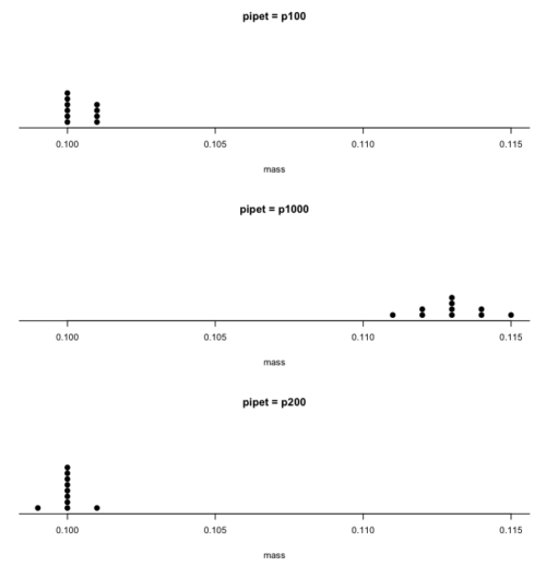
Figure 1. Dot plot of pipet results.
Note 2: Dotplot() is part of the RcmdrMisc package; if you are using the Rcmdr script window (please do!), then the functions in RcmdrMisc are already available and you wouldn’t need to use RcmdrMisc:: (package name plus double-colon operator) to call the Dotplot() function (more properly, referred to as namespaces). Thus, with(stackPipet, Dotplot(mass, by=pipet, bin=FALSE)) would work perfectly well within the Rcmdr script window.
From the dot plot we can quickly see that the p1000 was both inaccurate (the data fall well above the true value), and lacked precision (the values were spread about the mean value). The other two pipettors showed accuracy and looked to be similar in precision, although only two of ten values for the p200 were off target compared to four of ten values for the p100. Thus, we would conclude that the p200 was best at dispensing 100 microliters of water.
In the next chapter we apply statistics to estimate our confidence in this conclusion. In contrast to measurement, estimation implies calculation of a value. In statistics, estimates may be a point, e.g., a value of a collection of data, or an interval, e.g., a confidence interval.
Summary.
This is your first introduction into the concept of experimental design, as defined by statisticians! One of the key tasks for a statistical analyst is to have an appreciation for measurement accuracy and precision as established in the experiment. Precise and accurate measurement levels determine how well questions about the experiment can be answered. At one extreme, if a measure is imprecise, but accurate, then it will be challenging to quantify differences between a control group and a treatment group. At the other extreme, if the measure is precise, but inaccurate, the danger would be differences between the treatment and control group may be more likely, even when the groups are truly not different!
Questions.
- List the types of error in measuring mRNA expression levels on a gene for a sampling of cells from biopsy of normal tissue and a biopsy of a tumor. Assume use of NEXGEN methods for measuring gene expression. Distinguish between technical errors and biological errors.
- If confidence interval are useful for estimating accuracy, what statistic do we call to quantify precision?
Quiz Chapter 3.4
Estimating parameters
Chapter 3 contents
9.3 – Yates continuity correction
Introduction
Yates continuity correction: Most statistical textbooks at this point will note that critical values in their table (or any chi-square table for that matter) are approximate, but don’t say why. We’ll make the same directive — you may need to make a correction to the  for low sample numbers. It’s not a secret, so here’s why.
We need to address a quirk of the test: the chi-square distribution is a continuous function (if you plotted it, all possible values between, say, 4 and 3 are possible). But the calculated statistics we get are discrete. In our HIV-HG co-infection problem from the previous subchapter, we got what appears to be an exact answer for P, but it is actually an approximation.
We’re really not evaluating our test statistic at the alpha levels we set out. This limitation of the goodness of fit statistic can be of some consequence — increases our chance to commit a Type I error — unless we make a slight correction for this discontinuity. The good news is that the does just fine for most df, but we do get concerned with it’s performance at df = 1 and for small samples.
Therefore, the advice is to use a correction if your calculated is close to the critical value for rejection/acceptance of the null hypothesis and you have only one df. Use the Yate’s continuity correction to standard calculation,  .
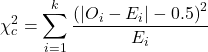
For the 2×2 table (Table 1), we can rewrite Yates correction

Our concern is this: without the correction, Pearson’s test statistic will be biased (eg, the test statistic will be larger than it “really” is), so we’ll end up rejecting the null hypothesis when we shouldn’t (that’s a Type I error). This becomes an issue for us when p-value is close to 5%, the nominal rejection level: what if p-value is 0.051? Or 0.049? How confident are we in concluding accept or reject null hypothesis, respectively?
I gave you three examples of goodness of fit and one contingency table example. You should be able to tell me which of these analyses it would be appropriate to apply to correction.
More about continuity corrections
Yates suggested his correction to Pearson’s back in 1934. Unsurprisingly, new approaches have been suggested (eg, discussion in Agresti 2001). For example, Nicola Serra (Serra 2018; Serra et al 2019) introduced
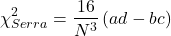
Serra reported favorable performance when sample size was small and the expected value in any cell was 5 or less.
R code
When you submit a 2X2 table with one or more cells less than five, you could elect to use a Fisher exact test, briefly introduced here (see section 9.5 for additional development), or, you may apply the Yates correction. Here’s some code to make this work in R.
Let’s say the problem looks like Table 1.
Table 1. Example 2X2 table with one cell with low frequency.
| Yes | No | |
| A | 8 | 12 |
| B | 3 | 22 |
At the R prompt type the following
library(abind, pos=15)
#abind allows you to combine matrices into single arrays
.Table <- matrix(c(8,12,3,22), 2, 2, byrow=TRUE)
rownames(.Table) <- c('A', 'B')
colnames(.Table) <- c('Yes', 'No') # when you submit, R replies with the following table
.Table  # Counts
 Yes No
A  8 12
B  3 22
Here’s the command; the default is no Yates correction (ie, correct=FALSE); to apply the Yates correction, set correct=TRUE.
.Test <- chisq.test(.Table, correct=TRUE)
Output from R follows
.Test
    Pearson's Chi-squared test with Yates' continuity correction
data:  .Table
X-squared = 3.3224, df = 1, p-value = 0.06834
Compare without the Yates correction
.Test <- chisq.test(.Table, correct=FALSE)
.Test
    Pearson's Chi-squared test
data:  .Table
X-squared = 4.7166, df = 1, p-value = 0.02987
Note that we would reach different conclusions! If we ignored the potential bias of the un-corrected we would be tempted to reject the null hypothesis, when in fact, the better answer is not to reject because Yates-corrected p-value is greater than 5%.
Just to complete the work, what does the Fisher Exact test results look like (see section 9.5)?
fisher.test(.Table)
    Fisher's Exact Test for Count Data
data:  .Table
p-value = 0.04086
alternative hypothesis: true odds ratio is not equal to 1
95 percent confidence interval:
0.9130455 32.8057866
sample estimates:
odds ratio
  4.708908
Which to use? The Fisher exact test is just that, an exact test of the hypothesis. All possible outcomes are evaluated and we interpret the results as likely as p=0.04086 if there is actually no association between the treatment (A vs B) and the outcome (Yes/No) (see section 9.5).
Questions
- With respect to interpreting results from a test for small samples, why use the Yates continuity correction?
- Try your hand at the following four contingency tables (a – d). Calculate the test, with and without the Yates correction. Make note of the p-value from each and note any trends.
(a)
| Yes | No | |
| A | 18 | 6 |
| B | 3 | 8 |
(b)
| Yes | No | |
| A | 10 | 12 |
| B | 3 | 14 |
(c)
| Yes | No | |
| A | 5 | 12 |
| B | 12 | 18 |
(d)
| Yes | No | |
| A | 8 | 12 |
| B | 3 | 3 |
3. Ch09.1, Question 1 provided an example of a count from a small bag of M&Ms. Apply the Yates correction to obtain a better estimate of p-value for the problem. The data were four blue, two brown, one green, three orange, four red, and two yellow candies.
- Construct a table and compare p-values obtained with and without the Yates correction. Note any trend in p-value
Quiz Chapter 9.3
Yates continuity correction
Chapter 9 contents
5.5 – Importance of randomization in experimental design
Introduction
If the goal of the research is to make general, evidenced-based statements about causes of disease or other conditions of concern to the researcher, then how the subjects are selected for study directly impacts our ability to make generalizable conclusions. The most important concept to learn about inference in statistical science is that your sample of subjects upon which all measurements and treatments are conducted, ideally should be a random selection of individuals from a well-defined reference population.
The primary benefit of random sampling is that it strengthens our confidence in the links between cause and effect. Often after an intervention trial is complete, differences among the treatment groups will be observed. Groups of subjects who participated in sixteen weeks of “vigorous” aerobic exercise training show reduced systolic blood pressure compared to those subjects who engaged in light exercise for the same period of time (Cox et al 1996). But how do we know that exercise training caused the difference in blood pressure between the two treatment groups? Couldn’t the differences be explained by chance differences in the subjects? Age, body mass index (BMI), overall health, family history, etc?
How can we account for these additional differences among the subjects? If you are thinking like an experimental biologist, then the word “control” is likely coming to the foreground. Why not design a study in which all 60 subjects are the same age, the same BMI, the same general health, the same family … history…? Hmm. That does not work. Even if you decide to control age, BMI, and general health categories, you can imagine the increased effort and cost to the project in trying to recruit subjects based on such narrow criteria. So, control per se is not the general answer.
If done properly, random sampling makes these alternative explanations less likely. Random sampling implies that other factors that may causally contribute to differences in the measured outcome, but themselves are not measured or included as a focus of the research study, should be the same, on average, among our different treatment groups. The practical benefits of proper random sampling is that recruiting subjects gets easier — fewer subjects will be needed because you are not trying to control dozens of factors that may (or may not!) contribute to differences in your outcome variable. The downside to random sampling is that the variability of the outcomes within your treatment groups will tends to increase. As we will see when we get to statistical inference, large variability within groups will make it less likely that any statistical difference between the treatment groups will be observed.
Demonstrate the benefits of random sampling as a method to control for extraneous factors.
The study reported by Cox et al included 60 obese men between the ages of 20 and 50. A reasonable experimental design decision would suggest that the 60 subjects be split into the two treatment groups such that both groups had 30 subjects for a balanced design. Subjects who met all of the research criteria and who had signed the informed consent agreement are to be placed into the treatment groups and there are many ways that group assignment could be accomplished. One possibility, the researchers could assign the first 30 people that came into the lab to the Vigorous exercise group and the remaining 30 then would be assigned to the Light exercise group. Intuitively I think we would all agree that this is a suspect way to design an experiment, but more importantly, why shouldn’t you use this convenient method?
Just for argument’s sake, imagine that their subjects came in one at a time, and, coincidentally, they did so by age. The first person was age 21, the second was 22, and so on up to the 30th person who was 50. Then, the next group came in, again, coincidentally in order of ascending age. If you calculate the simple average age for each group you will find that they are identical (35.5 years). On the surface, this looks like we have controlled for age: both treatment groups have subjects that are the same age. A second option is to sort the subjects into the two treatment groups so that a 21 year old is in Group A, and the other 21 year old is in Group B, and so on. Again, the average age of Group A subjects and of Group B subjects would be the same and therefore controlled with respect to any covariation between age and change in blood pressure. However, there are other variables that may covary with blood pressure, and by controlling one, we would need to control the others. Randomization provides a better way.
I will demonstrate how randomization tends to distribute the values in such a way that the groups will not differ appreciably for the nuisance variables like age and BMI differences and, by extension, any other covariable. The R work is attached following the Reading list. The take-home message: After randomly selecting subjects for assignment to the treatment groups, the apparent differences between Group A and Group B for both age and BMI are substantially diminished. No attempt to match by age and by BMI is necessary. The numbers are shown in the table and then in two graphics (Fig 1, Fig 2) derived from the table.
Table 1. Mean age and BMI for subjects in two treatment groups A and B where subjects were assigned randomly or by convenience to treatment groups.
| Group | Random assignment of subjects to treatment groups | Convenience assignment of subjects to treatment groups |
|---|---|---|
| A | 35.2 | 28 |
| B | 35.8 | 43 |
| A | 32.49 | 28.99 |
| B | 32.87 | 37.37 |
Just for emphasis, the means from Table 1 are presented in the next two figures (Fig 1 and Fig 2).
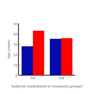
Figure 1. Age of subjects by groups (A = blue, B = red) with and without randomized assignment of subjects to treatment groups.
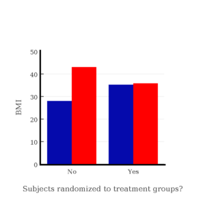
Figure 2. BMI of subjects by groups (A = blue, B = red) with and without randomized assignment of subjects to treatment groups.
Note that the apparent difference between A and B for BMI disappear once proper randomization of subjects was accomplished. In conclusion, a random sample is an approach to experimental design that helps to reduce the influence other factors may have on the outcome variable (eg, change in blood pressure after 16 weeks of exercise). In principle, randomization should protect a project because, on average, these influences will be represented randomly for the two groups of individuals. This reasoning extends to unmeasured and unknown causal factors as well.
This discussion was illustrated by random assignment of subjects to treatment groups. The same logic applies to how to select subjects from a population. If the sampling is large enough, then a random sample of subjects will tend to be representative of the variability of the outcome variable for the population and representative also of the additional and unmeasured cofactors that may contribute to the variability of the outcome variable.
What about observational studies? How does randomization work?
However, if you do cannot obtain a random sample, then conclusions reached may be sample-specific, biased. …perhaps the group of individuals that likes to exercise on treadmills just happens to have a higher cardiac output because they are larger than the individuals that like to exercise on bicycles. This nonrandom sample, an example of confounding where an extraneous or nuisance variable, body size, is associated with both the independent variable (exercise preference) and the dependent variable (cardiac output), will bias your results and can lead to incorrect interpretation of results.
Alternatively, perhaps a researcher elects to study the cardiac output of treadmill users versus bicycle users. The researcher sets up their testing station inside a gym’s powerlifting zone, where the largest individuals in the gym hang out. Inevitably because of this choice, the researcher over recruits larger individuals into the treadmill group, leading to a falsely elevated average cardiac output for treadmill users. This is an example of ascertainment bias — the sample is not representative of all treadmill users at the gym.
Random sampling is CRUCIAL in epidemiology, opinion survey work, most aspects of health, drug studies, medical work with human subjects. It’s difficult and very costly to do… so most surveys you hear about, especially polls reported from Internet sites, are NOT conducted using random sampling (included in the catch-all term “probability sampling“)!! As an aside, most opinion survey work involves complex sample designs involving some form of geographic clustering (eg, all phone numbers in a city, random sample among neighborhoods).
Random sampling is the ideal if generalizations are to be made about data, but strictly random sampling is not appropriate for all kinds of studies. Consider the question of whether or not EMF exposure is a risk factor for developing cancer (Pool 1990). These kinds of studies are observational: at least in principle, we wouldn’t expect that housing and therefore exposure to EMF is manipulated (cf. discussion Walker 2009). Thus, epidemiologists will look for patterns: if EMF exposure is linked to cancer, then more cases of cancer should occur near EMF sources compared to areas distant from EMF sources. Thus, the hypothesis is that an association between EMF exposure and cancer occurs non-randomly, whereas cancers occurring in people not exposed to EMF are random. Unfortunately, clusters can occur even if the process that generates the data is random.
Compare Graph A and Graph B (Fig 3). One of the graphs resulted from a random process and the other was generated by a non-random process. Note that the claim can be rephrased about the probability that each grid has a point, eg, it’s like Heads/Tails of 16 tosses of a coin. We can see clusters of points in Graph B; Graph A lacks obvious clusters of points — there is a point in each of the 16 cells of the grid. Although both patterns could be random, the correct answer in this case is Graph B.
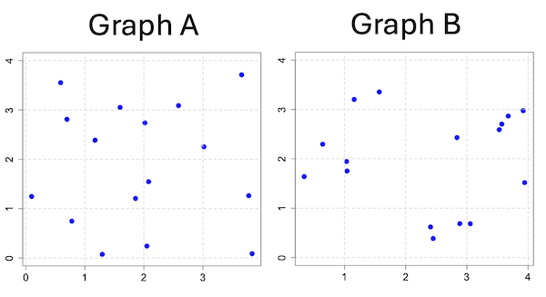
Figure 3. An example of clustering resulting from a random sampling process (Graph B). In contrast, Graph A was generated so that a point was located within each grid.
Hard to tell — and truth be told, random process could generate either one. To convince you, Figure 4 reveals the grouping that was done for Group A, in contrast with Group B which was drawn with the truly random process.
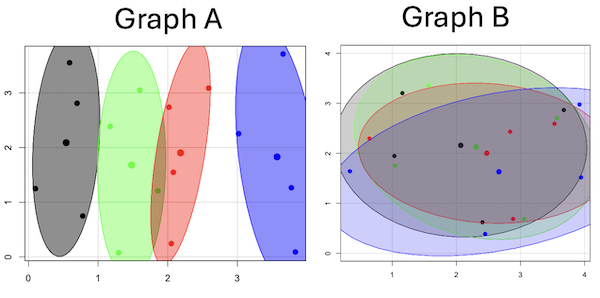
Figure 4. Same graphs as Figure 3, but with ellipses around the grouped data (hard to tell, but the centroids are the larger points).
Implications for sampling
The graphic below shows the transmission grid in the continental United States (Fig 5). How would one design a random sampling scheme overlaid against the obviously heterogeneous distribution of the grid itself? If a random sample was drawn, chances are good that no population would be near a grid in many of the western states, but in contrast, the likelihood would increase in the eastern portion of the United States where the population and therefore transmission grid is more densely placed.

Figure 5. Map of electrical transmission grid for continental United States of America. Image source https://openinframap.org/#3/24.61/-101.16
For example, you want to test whether or not EMF affects human health, and your particular interest is in whether or not there exists a relationship between living close to high voltage towers or transfer stations and brain cancer. How does one design a study, keeping in mind the importance of randomization for our ability to generalize and assign causation? This is a part of epidemiology which strives to detect whether clusters of disease are related to some environmental source. It is an extremely difficult challenge. For the record, no clear link to EMF and cancer has been found, but reports do appear from time to time (eg, report on a cluster of breast cancer in men working in office adjacent to high EMF, Milham 2004).
Questions
1. Use the sample() with and without replacement on the object (see help with R below)
fruit <- c("apple", "banana", "grape", "kiwi", "pear", "pineapple", "tomato")a) set of 3
b) set of 4
2. Confirm the claim by calculating the probability of Graph A result vs Graph B result (see R script below).
Quiz Chapter 5.5
Importance of randomization in experimental design
R code!
Code you type is shown in red; responses or output from R are shown in blue. Recall that statements preceded by the hash # are comments and are not read by R (ie, no need for you to type them).
First, create some variables. Vectors aa and bb contain my two age sequences.
 aa = seq(21,50)
 bb = seq(21,50)
Second, append vector bb to the end of vector aa
 age = append(aa,bb)
 age           #submit the vector (variable) name to print the records for verification - looks good!
  [1] 21 22 23 24 25 26 27 28 29 30 31 32 33 34 35 36 37 38 39 40 41 42 43 44 45 46 47 48 49 50 21 22 23 24 25 26 27 28 29 30 31 32 33 34 35 36 37
 [48] 38 39 40 41 42 43 44 45 46 47 48 49 50
Third, get the average age for the first group (the aa sequence) and for the second group (the bb sequence). Lots of ways to do this, I made a two subsets from the combined age variable; could have just as easily taken the mean of aa and the mean of bb (same thing!).
 A = age[1:30]
 mean(A)
 [1] 35.5
 B = age[31:60]
 mean(B)
 [1] 35.5
Fourth, start building a data frame, then sort it by age. Will be adding additional variables to this data frame
 ex.random = data.frame(age)
 AO.all = sort(ex.random$age)
 AO.age           #submit the vector (variable) name to print the records for verification - looks good!
  [1] 21 21 22 22 23 23 24 24 25 25 26 26 27 27 28 28 29 29 30 30 31 31 32 32 33 33 34 34 35 35 36 36 37 37 38 38 39 39 40 40 41 41 42 42 43 43 44
 [48] 44 45 45 46 46 47 47 48 48 49 49 50 50
Fifth, divide the variable again into two subsets of 30 and get the averages
 AO = AO.age[1:30]
 AO
  [1] 21 21 22 22 23 23 24 24 25 25 26 26 27 27 28 28 29 29 30 30 31 31 32 32 33 33 34 34 35 35
 mean(AO)
 [1] 28
 BO = AO.age[31:60]
 BO
  [1] 36 36 37 37 38 38 39 39 40 40 41 41 42 42 43 43 44 44 45 45 46 46 47 47 48 48 49 49 50 50
 mean(BO)
 [1] 43
Sixth, create an index variable, random order without replacement
rand.index = sample(1:60,60,replace=F)Add the new variable to our existing data frame, then print it to check that all is well
 ex.random$rand = rand.index
 ex.random
    age rand
 1   21   43
 2   22   15
 3   23   17
 4   24   35
 5   25   19
 6   26   18
 7   27   22
 8   28   31
 9   29   12
 10  30   44
 11  31   24
 12  32    5
 13  33    2
 14  34   50
 15  35   23
 16  36   20
 17  37   41
 18  38   56
 19  39   36
 20  40    8
 21  41   45
 22  42   38
 23  43   42
 24  44   46
 25  45   16
 26  46   21
 27  47   28
 28  48   10
 29  49   32
 30  50   54
 31  21   57
 32  22   51
 33  23   27
 34  24   40
 35  25   14
 36  26   48
 37  27   26
 38  28   58
 39  29    9
 40  30   11
 41  31    4
 42  32   52
 43  33   37
 44  34   53
 45  35    6
 46  36   34
 47  37   39
 48  38    7
 49  39    1
 50  40   47
 51  41   33
 52  42   60
 53  43   49
 54  44   30
 55  45   29
 56  46   55
 57  47   13
 58  48    3
 59  49   25
 60  50   59
Seventh, select for our first treatment group the first 30 subjects from the randomized index. There are again other ways to do this, but sorting on the index variable means that the subject order will be change too.
AR.age = ex.random[order(ex.random$rand),] #created a new data frame to distinguish it from the presorted version "ex.random"Print the new data frame to confirm that the sorting worked. It did. we can see that the rows have been sorted by ascending order based on the index variable.
 AR.age
    age rand
 49  39    1
 13  33    2
 58  48    3
 41  31    4
 12  32    5
 45  35    6
 48  38    7
 20  40    8
 39  29    9
 28  48   10
 40  30   11
 9   29   12
 57  47   13
 35  25   14
 2   22   15
 25  45   16
 3   23   17
 6   26   18
 5   25   19
 16  36   20
 26  46   21
 7   27   22
 15  35   23
 11  31   24
 59  49   25
 37  27   26
 33  23   27
 27  47   28
 55  45   29
 54  44   30
 8   28   31
 29  49   32
 51  41   33
 46  36   34
 4   24   35
 19  39   36
 43  33   37
 22  42   38
 47  37   39
 34  24   40
 17  37   41
 23  43   42
 1   21   43
 10  30   44
 21  41   45
 24  44   46
 50  40   47
 36  26   48
 53  43   49
 14  34   50
 32  22   51
 42  32   52
 44  34   53
 30  50   54
 56  46   55
 18  38   56
 31  21   57
 38  28   58
 60  50   59
 52  42   60
Eighth, create our new treatment groups, again of n = 30 each, then get the means ages for each group.
 AR = AR.age$age[1:30]
 mean(AR)
 [1] 35.16667
 AR2 = AR.all$all[31:60]
 mean(AR2)
 [1] 35.83333
Get the minimum and maximum values for the groups
 min(AR)
 [1] 22
 min(AR2)
 [1] 21
 max(AR)
 [1] 49
 max(AR2)
 [1] 50
Ninth, create a BMI variable drawn from a normal distribution with coefficient of variation equal to 20%. The first group with we will call cc
cc = rnorm(n=30,m=27.5, sd=5.5) #mean was 27.5 for this group with standard deviation of 5.5The second group called dd
dd = rnorm(n=30,m=37.5, sd=7.5) #mean was 37.5 for this group with standard deviation of 7.5Create a new variable called BMI by joining cc and dd
 BMI=append(cc,dd)
 BMI            #print out BMI to confirm. Looks good!
  [1] 27.87528 27.83250 31.88703 34.99041 24.06751 23.50952 22.57779 31.48394 31.04321 25.60258 25.41081 22.34619 34.62213 36.41348 41.17740
 [16] 20.56529 27.25238 21.85205 32.11690 32.37168 23.11314 33.29110 34.99106 38.22016 18.72105 26.22030 25.13412 27.50475 34.79361 32.81267
 [31] 47.57872 27.58428 40.17211 38.22195 26.91893 37.02784 53.72671 34.94727 30.35245 38.32571 40.52111 36.15627 30.36592 36.20397 47.63142
 [46] 40.30846 36.47643 50.86804 43.63741 37.84994 42.82665 41.71008 28.44976 24.57906 42.37762 38.38512 35.22879 31.34063 34.02996 27.28038
Add the BMI variable to our data frame.
 ex.random$BMI = BMI
 ex.random              #Print out the revised data frame. Looks good. We now have three variables: age, the index "rand," and now BMI
    age rand      BMI
 1   21   43 27.87528
 2   22   15 27.83250
 3   23   17 31.88703
 4   24   35 34.99041
 5   25   19 24.06751
 6   26   18 23.50952
 7   27   22 22.57779
 8   28   31 31.48394
 9   29   12 31.04321
 10  30   44 25.60258
 11  31   24 25.41081
 12  32    5 22.34619
 13  33    2 34.62213
 14  34   50 36.41348
 15  35   23 41.17740
 16  36   20 20.56529
 17  37   41 27.25238
 18  38   56 21.85205
 19  39   36 32.11690
 20  40    8 32.37168
 21  41   45 23.11314
 22  42   38 33.29110
 23  43   42 34.99106
 24  44   46 38.22016
 25  45   16 18.72105
 26  46   21 26.22030
 27  47   28 25.13412
 28  48   10 27.50475
 29  49   32 34.79361
 30  50   54 32.81267
 31  21   57 47.57872
 32  22   51 27.58428
 33  23   27 40.17211
 34  24   40 38.22195
 35  25   14 26.91893
 36  26   48 37.02784
 37  27   26 53.72671
 38  28   58 34.94727
 39  29    9 30.35245
 40  30   11 38.32571
 41  31    4 40.52111
 42  32   52 36.15627
 43  33   37 30.36592
 44  34   53 36.20397
 45  35    6 47.63142
 46  36   34 40.30846
 47  37   39 36.47643
 48  38    7 50.86804
 49  39    1 43.63741
 50  40   47 37.84994
 51  41   33 42.82665
 52  42   60 41.71008
 53  43   49 28.44976
 54  44   30 24.57906
 55  45   29 42.37762
 56  46   55 38.38512
 57  47   13 35.22879
 58  48    3 31.34063
 59  49   25 34.02996
 60  50   59 27.28038
Tenth, repeat our protocol from before: Set up two groups each with 30 subjects, calculate the means for the variables and then sort by the random index and get the new group means.
 AO = ex.random$BMI[1:30]
 mean(AO)
 [1] 28.99333
 BO = ex.random$BMI[31:60]
 mean(BO)
 [1] 37.36943
All we did was confirm that the unsorted groups had mean BMI of around 27.5 and 37.5 respectively. Now, proceed to sort by the random index variable. Go ahead and create a new data frame
 AR.age = ex.random[order(ex.random$rand),]
 AR.age                 #Print out the new data frame to confirm. Looks good.
    age rand      BMI
 49  39    1 43.63741
 13  33    2 34.62213
 58  48    3 31.34063
 41  31    4 40.52111
 12  32    5 22.34619
 45  35    6 47.63142
 48  38    7 50.86804
 20  40    8 32.37168
 39  29    9 30.35245
 28  48   10 27.50475
 40  30   11 38.32571
 9   29   12 31.04321
 57  47   13 35.22879
 35  25   14 26.91893
 2   22   15 27.83250
 25  45   16 18.72105
 3   23   17 31.88703
 6   26   18 23.50952
 5   25   19 24.06751
 16  36   20 20.56529
 26  46   21 26.22030
 7   27   22 22.57779
 15  35   23 41.17740
 11  31   24 25.41081
 59  49   25 34.02996
 37  27   26 53.72671
 33  23   27 40.17211
 27  47   28 25.13412
 55  45   29 42.37762
 54  44   30 24.57906
 8   28   31 31.48394
 29  49   32 34.79361
 51  41   33 42.82665
 46  36   34 40.30846
 4   24   35 34.99041
 19  39   36 32.11690
 43  33   37 30.36592
 22  42   38 33.29110
 47  37   39 36.47643
 34  24   40 38.22195
 17  37   41 27.25238
 23  43   42 34.99106
 1   21   43 27.87528
 10  30   44 25.60258
 21  41   45 23.11314
 24  44   46 38.22016
 50  40   47 37.84994
 36  26   48 37.02784
 53  43   49 28.44976
 14  34   50 36.41348
 32  22   51 27.58428
 42  32   52 36.15627
 44  34   53 36.20397
 30  50   54 32.81267
 56  46   55 38.38512
 18  38   56 21.85205
 31  21   57 47.57872
 38  28   58 34.94727
 60  50   59 27.28038
 52  42   60 41.71008
Get the means of the new groups
 AR = AR.age$BMI[1:30]
 mean(AR)
 [1] 32.49004
 min(AR)
 [1] 18.72105
 max(AR)
 [1] 53.72671
 AR2 = AR.all$BMI[31:60]
 mean(AR2)
 [1] 33.87273
 min(AR2)
 [1] 21.85205
 max(AR2)
 [1] 47.57872
That’s all of the work!
Data set
nonrandom
| X | Y |
| 0.779 | 0.747 |
| 0.098 | 1.248 |
| 0.697 | 2.811 |
| 0.59 | 3.553 |
| 1.295 | 0.075 |
| 1.858 | 1.207 |
| 1.172 | 2.388 |
| 1.597 | 3.051 |
| 2.051 | 0.242 |
| 2.081 | 1.546 |
| 2.016 | 2.738 |
| 2.587 | 3.088 |
| 3.833 | 0.088 |
| 3.776 | 1.264 |
| 3.017 | 2.254 |
| 3.657 | 3.712 |
random
| X1 | Y1 |
| 1.157 | 3.203 |
| 2.407 | 0.62 |
| 1.033 | 1.946 |
| 3.676 | 2.866 |
| 3.57 | 2.703 |
| 3.056 | 0.685 |
| 1.568 | 3.355 |
| 1.041 | 1.753 |
| 0.643 | 2.295 |
| 2.884 | 0.687 |
| 3.53 | 2.591 |
| 2.838 | 2.431 |
| 3.945 | 1.518 |
| 0.34 | 1.64 |
| 2.45 | 0.386 |
| 3.921 | 2.976 |
Chapter 5 contents
- The basics explained
- Experiments
- Experimental and Sampling units
- Replication, Bias, and Nuisance Variables
- Clinical trials
- Importance of randomization in experimental design
- Sampling from Populations
- References and suggested readings
5.3 – Replication, Bias, and Nuisance Variables
Introduction
This page describes additional elements of experimental design, replication and bias, which can impact the validity of a study.
Replication in science refers to repeating an experiment under identical conditions multiple times. To the extent the same conclusions are achieved, we can say the outcome is reproducible (Simmons 2014) and, therefore, likely to be objectively true (Earp 2011). Replication of experimental and sampling units is an essential component of good experimental design. Confusing technical replicates for biological replicates is called pseudoreplication.
Bias refers to any of a number of sociological and cognitive errors which may influence conclusions in science (Ionnidis 2005). In a meta-analysis, Fanelli et al (2017) reported that while the size of effect from identifiable biases were small, some disciplines were more prone to these sources of error. That researchers testing similar hypotheses reach different conclusions may result from bias. One such bias is positive outcome bias, where reports of null hypotheses are more often rejected than they should be based on sample size and other concerns of statistical power (see Chapter 11 – Power analysis).
The page concludes with a discussion of nuisance variables, variables that may be causally associated with the outcome of interest, but themselves are either of no interest in the study, or may not be known in advance (Meehl 1970; see also discussion of spurious correlations in Chapter 16.3 – Data aggregation and correlation).
Technical vs. biological replicates.
A laboratory technician retrieves a vial of an immortalized cell line from cryostorage and initiate propagation of the cells for the week’s work. After a couple of days of subculturing, the technician has grown millions of cells and is ready to set up an assay. After washing the cells in PBS (phosphate buffered saline), the technician adjusts the concentration of cells to 10,000 per mL media, places the tube on ice, and proceeds to set up a 48 well microplate. To each well, the technician adds media, one or more agents (Table 1), plus cells, total volume each well at one mL, three replicates per treatment.
Table 1. In our example there were four treatments plus a control (media only)
- DMSO only (D)
- DMSO + Cytokine (DC)
- DMSO + Small molecule Inhibitor (DS)
- DMSO + Cytokine + Small molecule Inhibitor (DCS)
- Media only (M)
The plate table might look something like Figure 1.

Figure 1. Schematics of a set up for a hypothetical 48 well microplate (plate_plot() from ggplate package).
The technician has done a lot of work; but, from a statistician’s point of view, effectively the technician has but one sampling unit to show for his efforts; one biological sampling unit because as far as we can tell, the cells were all related. Biological replication refers to repeat measures (eg, same conditions) on biologically distinct entities (Blainey et al 2014). Technical replication, in contrast, refers to repeat measures on the same entity, eg, the same individual (Blainey et al 2014).
However, there were more than one technical samples in the experimental design, twelve in all because there were twelve wells. Many of you will recognize this as the distinction between technical and biological replicates. In thinking about experimental design replicates pertain to the number of sampling units that are treated the same way. In our example cells may be “treated the same way” in at least two distinct ways. Biologically, the cells may be the same: derived from the same clonal cell, all at the same passage (generation) number, each cell genetically, morphologically, physiologically (etc.,) identical to the next cell. Technical replication on the other hand pertains to the levels of the treatments.
Within each of these treatments we had three wells, and that’s at the level of the technical replication.
A final note on this experiment. We as molecular biologists call each of these treatment groups, but statisticians thinking of this design would recognize only one treatment (called in statistics a factor), with four levels of the treatment. We will discuss this beginning in chapter 12 when we introduce analysis of variance.
Types of bias.
When we make decisions, we like to think we are rational; that we make decisions based on an evaluation of evidence. And yet, an increasing body of literature suggests that our decisions often made in a manner that falls short of rational processing. We outlined some sources of bias in Chapter 2.6. Deviance from rational decision making is due to any number of cognitive biases we may have. Researchers and medical doctors make many decisions and, unfortunately, are just as susceptible to cognitive biases as the rest of us. One kind of bias that is bedeviling to research is confirmatory bias. Confirmatory bias refers to a researcher in effect seeking evidence in a way that confirms a prior conclusion (Kaptchuck 2003). Confirmatory bias would be exhibited if we report positive effects of aspirin to relieve migraines in subjects, but exclude cases where the subjects report no improvement. Medical doctors may be risk averse and therefore tend to over-prescribe, or they may be risk-takers (eg, rise and fall of high-dose chemotherapy, cf, discussion in Howard et al. 2011).
The concept of bias was first introduced in Chapter 3 and will be returned to in subsequent chapters. In general, bias refers to the objectivity of measurement and inferences about such measurements. Bias implies that a series of measurements consistently fail to return the true value of the variable. Bias is systematic error and may be associated with a poorly calibrated instrument or even the use of improper sets of rules for measurement given the nature of the characteristic. Bias can be captured by the concept of accuracy.
Bias is challenging to eliminate; the best way is to design the experiment so that the observer, the researcher, is unaware of the specific questions to be tested. The research is conducted “blind.” Clinical research provides the easiest examples. A trial can be blind in a couple of ways:
- The subjects do not know which treatment they receive, but the researcher does know
- The researcher does not know which treatment subjects receive, but the subjects know
- Neither the researcher nor the subjects know which treatment they receive.
- The other possibility is that both the researcher and the subjects know treatments received — this would be a poor design.
Bias can enter a research project at multiple levels. A partial list of sources of bias in research includes (modified after Pannucci and Wikins 2010):
Bias that occurs before the experiment
- Inadequate planning of the experiment, flawed design
- Bias in selection of subjects from the reference population
- Surveillance bias, where one group is studied more closely than another group.
Surveillance bias, also called detection bias or ascertainment bias, a type of information bias. Characterized as “the more you look, the more you find (Sackett 1979),” differences in outcome counts varies with differences in effort to detect. Recently, cases of myocarditis in young people were reported following Covid-19 mRNA vaccination (eg, Bozkurt et al 2021. Marshall et al 2021). However, myocarditis reports following vaccination occur at the rates expected in the population, and the reports lack important context (eg, other respiratory viruses known to cause myocarditis not ruled out), suggesting the putative link between Covid-19 vaccines and this heart condition may be result of us looking hard for signs of adverse effects of the vaccine (cf, discussion in O’Leary and Maldonado 2021).
Bias during the experiment
- Interviewer bias
- Chronology bias
- Recall bias
- Transfer bias
- Misclassification of exposure or outcome
- Performance bias
Performance bias refers to conditions of an experiment that introduce unintended differences between groups. For example, subjects enrolled in a weight-loss study randomly assigned to the control group may react poorly when they realize they are not receiving the experimental intervention. This leads to potential for a systematic bias — participants in the control group may behave differently, counteracting the point of randomization (McCambridge et al 2014).
Another well-known performance bias is associated with eliciting maximal performance from animals, such as running stamina or maximum sprint running speed (Losos et al 2002). For example, spring running speed of lizards may be measured by placing lizards onto a high-speed treadmill, then increasing belt speed to match the individual’s burst performance (eg, Dohm et al 1998). Clearly, not all individuals will perform to maximum physiological capabilities under these conditions.
Bias after the experiment
- Citation bias
- Confounding
Another way to view sources of bias is that, at least from the perspective of the researcher, the bias is likely to be unconscious bias. After all, if we knew about the sources of bias we would work our experiments in such a way to minimize known error producing sources (Holman et al 2015). Selecting subjects at random and keeping record keeping blind with respect to treatments are among the best tools we have to avoid this kind of bias.
Nuisance variables
A key quality of experimental design is the opportunity afforded the researcher to apply control. In a classic view of the experiment, one allows only one aspect to vary, the treatment applied, all else is controlled. Thus, any difference in outcome may be attributed to the treatment. However, it is likely impossible to control for all possible variables that may affect our outcome; confounding clear interpretation of results (see Chapter 16.2 and 16.3). Consider, for example, the effects of age on running performance (Fig. 2).
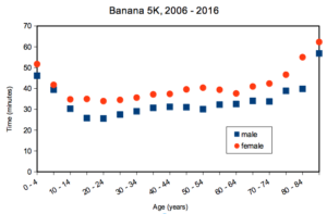
Figure 2. Mean 5K running times (minutes) by age and gender (2006 – 2016, Jamba Juice Banana 5K race, Honolulu, HI).
If we are interested in gender differences, we must also deal with the change in performance with age: older runners regardless of gender tend to run slower than younger runners. Thus, in the comparison of genders, age is a nuisance variable. In the literature, you may see “lurking variable,” or other such names. The concept is that these variables may be causal, but are either of no interest in the study, or may not be known in advance. Therefore, age must be accounted for before we can address gender differences, if any. Age, in this case, is considered a nuisance variable because we are not primarily interested in age effects, but age clearly covaries (is associated) with running performance. How best to handle nuisance variables? One approach is to match by age (blocking effect, see Chapter 14.4); another approach would be to randomly select with respect to age when compiling female and male times.
Another example of confounding. Results from ecological experiments intended to test for presence of competition for resources by plant species by removing plants may alter herbivory levels; thus, survivorship not the result of reduced plant-plant competition but because of changes in herbivore behavior (Reader 1992).
Questions
- I cite a number of articles in Mike’s Biostatistics Book. If you’re paying attention, you’ll have noticed that all of my citations, at least for articles, link to a source that you can either download or read online. What kind of error am I committing by following this approach?
- In large part because of the tendency for overuse of antibiotics, doctors are less likely today to prescribe antibiotics for patients with upper respiratory tract infections than in the past (Zoorob et al 2012). URTI are mostly caused by rhinovirus infections (Calderaro et al 2022) and, therefore, the course of infection in a patient should be unaffected by addition of antibiotic. However, although rare compared to URTI, life-threatening illness like acute epiglottitis caused by bacteria infection can sometimes develop or accompany URTI. Thus, not prescribing antibiotics at a diagnosis of URTI may risk a worsening condition for the patients. This sets the doctor up for a potential cognitive bias – to prescribe or not to prescribe antibiotics prophylactically? Discuss this decision in the context of potential sources of cognitive biases and possible outcomes of the decision.
Quiz Chapter 5.3
Replication, bias, and nuisance variables
Chapter 5 contents
- The basics explained
- Experiments
- Experimental and Sampling units
- Replication, Bias, and Nuisance Variables
- Clinical trials
- Importance of randomization in experimental design
- Sampling from Populations
- References and suggested readings
5 – Experimental design
Beyond numbers.
During this course, you will learn about statistics, yes, but my hope and goal for your experience in this class is much more than that: statistical reasoning. To have statistical reasoning skills, you need to be comfortable with the context of how data are acquired, ie, data acquisition. It’s not just about knowing how an instrument performs, eg, under or over the limits of quantification characteristics of the instrument lead to censored missing values, missing not at random (MNAR). In a broad stoke view, data are obtained from two kinds of studies: observational studies and experimental (manipulative) studies. what a correctly designed experiment can tell you about the world, and how a poorly designed experiment works against you. At the end of the semester, you should be familiar with the issues of Randomization, Control, Independence, and Replication.
The basics explained.
Experimental design is a discipline within statistics concerned with the analysis and design of experiments. Design is intended to help research create experiments such that cause and effect can be established from tests of the hypothesis. We introduced elements of experimental design in Chapter 2.4. I recommend a quick re-read: We talk about the different types of bias that can affect research. We also point out parts of the problem you’ll need to think about when planning a project, so you can avoid or reduce bias from the start.
Note 1: Just the highlights from Chapter 2.4: use randomization, blinding, and control measures in the study design. Different strategies may be needed depending on the type of bias.
Here, we expand our discussion of experimental design. We begin with review of definitions and an outline of an important concept in statistics. First, we need to be clear about why we measure or conduct experiments. We do so to collect data (datum is the singular) about a characteristic or trait from a population. Data are observations: they include observations and measurements from instruments. At their best, data are the “facts” of science.
Measurement, Observation, Variables, Values.
Measurement is how we as scientists acquire our data (Chapter 3.4). The process of measuring involves the assignment of numbers, codes, or labels to observations according to rules established prior to any data collection (Stevens 1946, Houle et al 2011). Observations refer to the units of measurement, whereas variables are the characteristics or traits that are measured. A value refers to the particular number, score, or label assigned to a particular sample for a variable. Variables are generic, the thing being measured, values are specific to the subject or sample being measured for the variable. Each discipline in biology has its own set of variables and samples may or may not have different values for each variable measured. Variables are summarized as a statistic (eg, the sample mean), which is a number taken to estimate a parameter, which pertains to the population. Variables and parameters in statistics were discussed in Chapter 3.4. Because numbers or scores or labels can be assigned according to different rules, this means that variables may be measured on different kinds of scales or data types. The different kinds of data types were presented in Chapter 3.1.
Missing values.
A missing value refers to lack of a value for an observation or variable (Chapter 3.5). Censored values, a type of missing value, include observations for which limited or partial information is available, eg, range, while a missing value lacks any information about the true value.
Missing values can affect analysis and many R algorithms are sensitive or may fail to run in the presence of missing values. Missing data may be of three kinds, and one of them, missing not at random (MNAR), can substantially influence the analysis. MNAR implies some observations are missing because of a systematic bias. Instrument limits of quantification are an example of systematic bias — for example, spectrophotometric absorbance readings of zero for a colorimetric assay (eg, Bradford protein assay) may not represent complete absence of the target, but rather, the lower detection limits of the instrument or the assay method (0.1 mg protein/mL in this case).
The other kinds of missing values are missing completely at random (MCAR) and missing at random (MAR). MCAR implies there is no association between any element of the experiment and the absence of a value. Analysis on MCAR data sets may support unbiased conclusions. MAR includes the random errors that occur during data acquisition: data may be lost because of operator error or power outage (shudder). Unlike MNAR, analysis of MAR, like MCAR data sets may still result in unbiased conclusions.
Note 2: The word “may” is doing some heavy lifting here; obviously, the size of the data set influences whether this claim holds.
One consequence of missing values — a decision how best to handle the lost information. The options are either pairwise deletion or listwise deletion. Listwise means the entire row, all variables, are lost for any record with one or more missing values. You recorded root length, stem length, numbers of secondary roots, time to germinate, but the SPAD meter failed and there is no chlorophyl reading for seedling #212? Sorry, the entire row is deleted. Optionally, the missing data is deleted pairwise — only chlorophyl reading for #212 is lost, all other variables remain.
Users of R will quickly learn some algorithms immediately fail to run if not instructed how to process missing values. In some cases, missing values can be replaced by imputed values.
Note 3: This being an introduction to applied biostatistics, we won’t dwell on the pros and cons of imputation. Instead, I point interested readers to two heavily cited articles: Schafer 1999; Schafer and Graham 2002.
Cause & Effect.
Observations or measurements gathered under controlled conditions (experiments) are essential if we are to answer questions about populations, to separate cause and effect, where one or more events is directly the result of another factor, as opposed to anecdote, a story about an event which, by itself, cannot be used to cause from association (eg, spurious correlations, see Ch 16.2). Recall that anecdotal evidence typically comes from personal experience, where observations may be obtained by non-systematic methods. Well designed experiments, in the classical sense, permit discrimination among competing hypotheses in large part because observations are collected according to strict rules. Well developed hypotheses tested by well-designed experiments permit ruling out alternative explanations (sensu Pratt [1964] strong inference). Observational studies, or epidemiology studies if we are talking about investigations of risk assessment, also may contribute to discussions of cause and effect (see history of smoking by Doll 1998).
Medicine is replete with stories about how a patient showed a particular set of symptoms, and how a physician applied a set of diagnostic protocols. An outcome was achieved, and the physician reports the outcome and circumstances related to the patient to her colleagues. This is an example of a case study, and the focus of investigation is the individual, the patient. The doctor’s report will sound like, “I tried the standard treatment given the diagnosis, and the patient’s symptoms diminished, but later returned. I tried a higher dose, but the patient’s symptoms persisted unabated.” No inferences are made to a wider set of individuals and the report is anecdotal. If observations are made on several patients, this may be a case series.
In ecology, a field biologist may notice a six-legged adult frog (Scott 1999, Alvarez et al 2021) — since frogs typically have four legs, the six-legged frog attracts the biologist’s eye and he jots down the circumstances in which the frog were found: relative humidity, air temperature, ground temperature, where the frogs was found (on lower leaf of a philodendron plant). A water source near where the frog was found is tested for pH with a meter the biologist carries, and a water sample is taken for later testing of herbicides. The frog is collected so that it can be checked for skin parasites. Upon further inspection, the frog did indeed have parasites known to cause deformities in other frog species. However, note that this example too, is a case study. Although the biologist makes additional observations, any conclusions about why the frog has six legs is anecdotal.
From these case studies, no conclusions can be drawn. We cannot say why the patient failed to respond to treatment, nor can we say why the frog has six legs. Why? Because these are singular events, and a variety of explanations can be given as to their causes — importantly, no controls are available, so there’s no way to distinguish among possibilities.
From such anecdotes, however, experiments can be designed. The physician may decide to recruit additional patients with the diagnosed illness and apply the standard treatment to see if her anecdote is a single, unique event, or more indicative of a problem with the treatment. The biologist may collect other frogs from the area near where he found the six-legged frog and check to see if they, too, have the parasites. If additional patients fail to respond to the treatment, then the singular even is more likely to be a phenomenon. If the normal frogs also have similar levels of the parasite then it is unlikely that these parasites caused the malformed frog. With this simple step (recruiting similar patients, finding additional frogs), we can begin to make inferences about cause and effect and in some cases, to generalize our findings.
This is the objective of most statistical procedures, the concept of sampling from a reference population and making distinctions between groups within the sample. The difference between observational and experimental studies then is how the subjects are selected with respect to the groups. In an experiment, the researcher controls and decides which subject receives the treatment, therefore, allocation to groups is manipulated by the researcher. In contrast, subjects included in an observational study have already been “assigned” to a group, but not by us. Assignment to groups, smokers or non smokers, Type II diabetes or no diabetes (etc.), is done by nature.
Now, I do not wish to imply that research that cannot be generalized back to a reference population are worthless. Far from it. In fact, there is a strong argument for specificity. For example, much basic biological research depends on work or model organisms, which in turn may be further partitioned into specific genetic lines (cf. discussion in Rothman et al 2013). And my goodness, what we have learned about the devastation to oceanic islands like Guam when the brown tree snake was introduced (Fritts and Rodda 1998). Strictly speaking, what has happened to Guam is a case history. But no one would argue that what has happened to Guam cannot happen to Hawaii and other oceanic islands (eg, United States Federal law 384-108 “Brown Tree Snake Control and Eradication Act of 2004”). In other words, even from case histories, generalizations can sometimes be made.
There can also be real reasons to ignore the issue of generality. One benefit of specificity is experimental control. Transgenic lines may differ by single gene knockout or by gene duplication, and clearly the aim of such studies is to evaluate the function (hence purpose) of the gene product (or its absence) on some phenotype. In this sense it may not seem important that an transgenic mouse is not representative of a wild outbred mouse population. However, this argument is fundamentally one of expedience — such studies do result in specific results, results that cannot be generalized beyond the strains involved. It ignores the issue of genetic background — all of the genes that affect a trait in addition to the candidate gene under study (Sigmund 2000; Lariviere et al 2001). Transgenic mice of different inbred strains or their hybrids may have very different alleles at other genes that may influence a phenotype, hence, the results of the gene knockdown or other engineering result in different outcomes. Results of genetic manipulations on inbred strains, no matter how sophisticated, the conclusions are strain- or hybrid cross-specific. Thus, although technically and financially difficult, conclusions are better, more generalizable, when conducted with many different inbred lines and verified in outbred mouse populations precisely because genetic background often influences function of single genes (Sigmund 2000; Lariviere et al 2001).
“Causal criteria:” Logic of causation in medicine.
This section is in progress. Just a list of key points and references
Throughout this text, emphasis on the power of experimentation is emphasized. Well designed experiments …
Henle-Koch’s postulates (1877, 1882), working on tuberculosis reported a set of causal criteria to establish link between a microorganism and a disease, are the following:
- The microorganism must be found in abundance in all organisms suffering from the disease, but should not be found in healthy organisms.
- The microorganism must be isolated from a diseased organism and grown in pure culture.
- The cultured microorganism should cause disease when introduced into a healthy organism.
- The microorganism must be reisolated from the inoculated, diseased experimental host and identified as being identical to the original specific causative agent.
Robert Koch wrote these more than 100 years ago, so, clearly, understanding of infectious disease has improved. Evan’s postulates, quoted from A Dictionary of Epidemiology, 5th edition (pp. 86-87).
- Prevalence of the disease should be significantly higher in those exposed to the hypothesized cause than in controls not so exposed.
- Exposure to the hypothesized cause should be more frequent among those with the disease than in controls without the disease—when all other risk factors are held constant.
- Incidence of the disease should be significantly higher in those exposed to the hypothesized cause than in those not so exposed, as shown by prospective studies.
- The disease should follow exposure to the hypothesized causative agent with a normal or log-normal distribution of incubation periods.
- A spectrum of host responses should follow exposure to the hypothesized agent along a logical biological gradient from mild to severe.
- A measurable host response following exposure to the hypothesized cause should have a high probability of appearing in those lacking this before exposure (eg, antibody, cancer cells) or should increase in magnitude if present before exposure. This response pattern should occur infrequently in persons not so exposed.
- Experimental reproduction of the disease should occur more frequently in animals or humans appropriately exposed to the hypothesized cause than in those not so exposed; this exposure may be deliberate in volunteers, experimentally induced in the laboratory, or may represent a regulation of natural exposure.
- Elimination or modification of the hypothesized cause should decrease the incidence of the disease (eg, attenuation of a virus, removal of tar from cigarettes).
- Prevention or modification of the host’s response on exposure to the hypothesized cause should decrease or eliminate the disease (eg, immunization, drugs to lower cholesterol, specific lymphocyte transfer factor in cancer).
- All of the relationships and findings should make biological and epidemiological sense.
Fredericks, D. N., & Relman, D. A. (1996). Sequence-based identification of microbial pathogens: a reconsideration of Koch’s postulates. Clinical microbiology reviews, 9(1), 18-33.
Correlation (association) does not imply causation, a well-worn truism in any application of critical thinking skills. Conversely, causation does imply association (correlation); If a change in one variable directly changes another variable, there will be a statistical association between the two variables. Thus, a correlation between two variables is necessary, but not sufficient evidence for cause and effect between two variables.
Note 4: Association is the more general term for a possible relationship between two or more variables. A correlation in statistics generally refers to a linear association (Chapter 16); the aforementioned truism should be restated as association (or statistical relationship) does not imply causation.
However, sometimes association does point to a cause. A familiar example is association between tobacco cigarette smoking causes lung cancer. Surgeon General Luthar Terry’s 1964 report (link to document in National Library of Medicine), presented a strong case linking smoking to elevated risk of lung cancer and coronary artery disease.
Bradford Hill’s guidelines to evaluate causal effects based on epidemiology (Hill 1965, see also Sussar 1999, Fedak et al 2015). Set of necessary and sufficient conditions, inductive reasoning.
- Strength of association
- Consistency of observed association
- Specificity of association
- Temporal relationship of the association
- Biological gradient, eg, a dose-response curve
- Biological plausibility
- Coherence, the cause and effect inference should not conflict with what is known about the etiology of a disease.
Follows and extends David Hume’s (1739) causation criteria: association (Hill #1), cause precedes effect (Hill #4), direction of connection.
Validity.
An obvious objective of research is to reach valid conclusions about fundamental questions. A helpful distinction between the specific and the generalizable experiment is to recognize there are two forms of validity in research: internal validity and external validity (Elwood 2013). Internal validity is the quality of a designed study that determines whether cause and effect can be determined. Random assignment of subjects to treatment groups enhances the internal validity of the study. External validity relates to how general the assessment of cause and effect can be to other populations. Thus, random sampling from a reference population has to do with whether or not the study has external validity.
Additional definitions.
We proceed now with definitions. We use the term population in a special and restrictive way in statistics. Our definition includes the one you are already familiar with, but it also means more than that.
Populations are the entire group of individuals that you want to investigate. In statistics, the entire groups is actually the entire class with the observation — so if we are referring to the average body weight of house mice, we’re actually referring to the body weight as the population — it’s a subtle distinction, not essential for our introduction to biostatistics. When we conduct experiments and apply statistical tests on collected data, we generally intend to make inferences (draw conclusions) from our results back to the population.
Population has a strict application in statistics, but the definition also includes our general understanding of the word population. For example, Examples of a population in the general sense one may refer to include: .… the entire human population existing today .… the entire collection of U.S. citizens. .… all the individuals in an entire species. .… all individuals in a population of a species (eg, house mice in a dairy barn in Hawai’i) .… all of us in this classroom (if we are ONLY interested in US) If you could measure the entire population then there would be no need to do (or learn) statistics! Populations usually are in the thousands, millions, or billions of individuals. Here, population is used in the everyday sense that we think of — a collection of individuals that share a characteristic.
A more formal definition of “population” in statistics reads as follows: A statistical population is the complete set of possible measurements on a trait or characteristic corresponding to the entire collection of sampling units for which conclusions are intended.
To conclude, in this class, when we talk about population, we will generally be using it in the everyday sense of the word. However, keep in mind that the definition is more restrictive than that and the key is to identify what sampling units are measured.
Conclusions.
This is only the beginning, the basics of experimental design. Beginning with RA Fisher‘s 1935 book, The Design of Experiments (nine editions, some freely accessible via internet search), which is still very much worth reading, entire books are written on the subject, as you can well imagine.
Note 5: Fisher’s The Design of Experiments concerned experimental design, randomization, blocking, and replication, particularly from perspective of agriculture research. Most readers of this eBook likely know that RA Fisher’s broader career absolutely included eugenics and hereditarian views about human populations and race. Those views are not in The Design of Experiments, which is largely about methods and statistical framework for inference.
We will also return to the subject of Experimental Design throughout the book. We will return to random sampling in Chapter 5.5. Next we discuss distinctions between experiments and observational studies with respect to sampling of populations.
A bit of a disclaimer here before proceeding; while I cite several papers for examples in experimental design in Chapter 5, reader’s should not read into this that I am either criticizing or endorsing the published experiments. Experimental design will always have elements of compromise — the trick of course is knowing which choices influence validity (Thompson and Panacek 2006).
Questions.
- Define in your own words the following terms
- reference population
- subjects
- specific versus general conclusions
- random sampling
- convenience sampling
- haphazard sampling
- research validity
- Revisit our cell experiment, “What is the sampling unit in the following cell experiment?” How would you change this experiment so that there will be biological and not just technical replication?
- Describe the type of sampling for each research scenario described?
- All African snails on a staircase at Chaminade University are collected on a Thursday evening.
- All African snails on a staircase at Chaminade University are collected every Thursday evening for six months.
- All African snails on all staircases at Chaminade University are collected.
- African snails are studied in the lab, then returned to the areas from which they were collected. Days later, the researcher collects snails from the same area.
- African snails are studied in the lab, then returned to the areas from which they were collected. Days later, the researcher collects snails from a different area.
- The Chaminade University campus is divided into grids. Grids that include stairwells are marked. Before collecting snails, the researcher randomly selects from the list of grids and searches for snails only in those grids selected from the list.
Figure 1. Giant African Snail (Lissachatina fulica, formerly Achatina fulica). Image by M. Dohm.
- This next scenario may be evaluated by you for potential sources of bias. Review the list of bias listed above. A researcher wants to do a population count of feral cats on campus. Feral cats are active at night, so he decides to set up a feeding station near a light post. The researcher sits all night in a parked car yards away and watches the feeding station for visits by cats. The researcher repeats these observations over the course of a week, moving the feeding station to different campus locations each night, and reports the total number of cats seen during the week as an estimate of the population size. Be able to discuss this study in terms of potential and actual bias.
Quiz
Including the quiz on this page, a total of 65 questions among the several subchapters, a mix of true or false and multiple choice question format.
Quiz Chapter 5
Experimental design
Chapter 5 contents
3.3 – Measures of dispersion
More about summary statistics.
The statistics of data exploration involve calculating estimates of the middle, central tendency, and the variability, or dispersion, about the middle. Statistics about the middle were presented in the previous section, Chapter 3.1. Statistics about measures of dispersion, and how to calculate them in R, are presented in this page. Use of Z score to standardize or normalize scores is introduced. Statistical bias is also introduced.
Describing the middle of the data gives your reader a sense of what was the typical observation for that variable. Next, your reader will want to know something about the variation about the middle value — what was the smallest value observed? What was the largest value observed? Were data widely scattered or clumped about the middle?
Measures of dispersion or variability are descriptive statistics used to answer these kinds of questions. Variability statistics are very important and we will use them throughout the course. A key descriptive statement of your data, how variable?
Note 1: Data is plural = a bunch of points or values; datum is the singular and rarely used.
Examine the two figures below (Fig 1 and Fig 2): the two sample frequency distributions (put data into several groups, from low to high, and membership is counted for each group) have similar central tendencies (mean), but they have different degrees of variability (standard deviation).
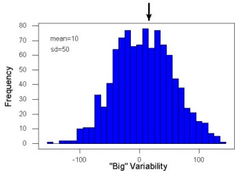
Figure 1. A histogram which displays a sampling of data with a mean of 10 (arrow marks the spot) and standard deviation (sd) of 50 units.
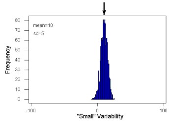
Figure 2. A histogram which displays a sampling of data with the same mean of 10 (arrow marks the spot) displayed in Fig. 1, but with a smaller standard deviation (sd) of 5 units.
Clearly, knowing something about the middle of a data set is only part of the required information we need when we explore a data set; we need measures of dispersion as well. Provided certain assumptions about the frequency of observations hold, estimates of the middle (eg, mean, median) and the dispersion (eg, standard deviation) are adequate to describe the properties of any observed data set.
For measures of dispersion or variability, the most common statistics are: Range, Mean Deviation, Variance, Standard Deviation, and Coefficient of Variation.
The range.
The range is reported as one number, the difference between maximum and minimum values.

Arrange the data from low to high, subtract the minimum, Xmin, from the maximum, Xmax, value and that’s the range.
For example, the minimum height of a collection of fern trees might be 1 meter whereas the maximum height might be 2.2 meters. Therefore, the range is 1.2 meters (= 2.2 – 1).
The range is useful, but may be misleading (as index of true variability in population) if there is one or more exceptional “outlier” (one individual that has an exceptionally large or small value). I often just report Xmin and Xmax. That’s the way R does it, too.
If you recall, we used the following as an example data set.
x = c(4,4,4,4,5,5,6,6,6,7,7,8,8,8,15)The command for range in R is simply range().
range(x)
[1] 4 15
There is apparently no universally accepted symbol for “range,” so we report the statistic as range = 15 – 4 = 11.
You may run into an interquartile range, which is abbreviated as IQR. It is a trimmed range, which means, like the trimmed mean, it will be robust to outlier observations. To calculate this statistic, divide the data into fourths, termed quartiles. For our example variable, x, we can get the quartiles in R
quantile(x)
  0%  25%  50%  75% 100%
 4.0  4.5  6.0  7.5 15.0
Thus, we see that 25% of the observations are 4.5 (or less), the second quartile is the median, and 75% of the observations are less than 7.5. The IQR is the difference between the first quartile, Q1, and the third quartile, Q3.
The command for obtaining the IQR in R is simply IQR(). Yes. You have to capitalize “IQR” — R is case sensitive; that means IqR is not the same as IQR or iqr.
IQR(x)
[1] 3.5
and we report the statistic as IQR = 3.5. Thus, 75% of the observations are within 3.5 points of the median. The IQR is used in box plots (Chapter 4). Quartiles are special cases of the more general quantile; quantiles divide up the range of values into groups with equal probabilities. For quartiles, four groups at 25% intervals. Other common quantiles include deciles (ten equal groups, 10% intervals) and percentiles (100 groups, 1% intervals).
The mean deviation.

Subtract each observation from the sample mean; each  is called a deviate: some observations will be positive (greater than
 ) and some will be negative (less than ).
Take the absolute value of the deviation and then add up the absolute values of the deviations from the mean. At the end, divide by the sample size, n. Large values for this statistic implies that much of the data is spread out, far from the mean. Small values in turn imply that each observation is close to the mean.
Note 2: The mean deviation will always be positive, which is why we take the absolute. By taking the absolute value of each deviate, then the sum is greater than zero. Now, we rarely use this statistic by itself — but that difference is integral to much of the statistical tests we will use. Look for this difference in other equations!
In R, we can get the mean deviation with the mad() function. At the R prompt, then
mad(x)
[1] 2.9652
Population variance and population standard deviation.
The population variance is appropriate for describing variability about the middle for a census. Again, a census implies every member of the population was measured. Equation of the population variance is
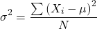
The population standard deviation also describes the variability about the middle, but has the advantage of being in the same units as the quantity (ie, no “squared” term). Equation of the population standard deviation is

Sample variance and sample standard deviation.
The above statements about the population variance and standard deviation hold for the sample statistics. Equation of the sample variance
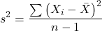
and the equation of the sample standard deviation

Of course, instead of taking the square-root of the sample variance, the sample standard deviation could be calculated directly.
*** QuickLaTeX cannot compile formula:
\begin{align*}s = \sqrt{\frac{\sum \left ( X_{i} - \bar{X} \right )^2}{n-1}\end{align*}

*** Error message:
File ended while scanning use of \align*.
Emergency stop.
n - 1 instead of N. This is Bessel’s correction and we will take a few moments here and in class to show you why this correction makes sense. Bessel’s correction to the sample variance illustrates a basic issue in statistics: when estimating something, we want the estimator (ie, the equation), to be an unbiased value for the population parameter it is intended to estimate.Statistical bias is an important concept in its own right; bias is a problem because it refers to a situation in which an estimator consistently returns a value different from the population parameter for which it is intended to estimate. Thus, the sample mean is said to be an unbiased estimator of the population mean. Here, bias means that the formula will give you a good estimate of the value. This turns out not to be the case for the sample variance if you divide by n instead of n - 1. Now, for very large values of n, this is not much of an issue, but it shows up when n is small. In R you get what you ask for — if you ask for the sample standard deviation, the software will return the correct value; calculators, go to watch out for this — not all of them are good at communicating which standard deviation they are calculating, the population or the sample standard deviation.
Winsorized variances.
Like the trimmed mean and winsorized mean (Ch3.2), we may need to construct a robust estimate of variability less sensitive to extreme outliers. Winsorized refers to procedures to replace extreme values in the sample with a smaller value. As noted in Chapter 3.2, we chose the level ahead of time, eg, 90%. Winsorized values then The winsorized variance is just the sample variance of the winsorized values. winvar() from the WRS2 package.
Making use of the sample standard deviation.
Given an estimate of the mean and an estimate of the standard deviation, one can quickly determine the kinds of observations made and how frequently they are expected to be found in a sample from a population (assuming a particular population distribution). For example, it is common in journal articles for authors to provide a table of summary statistics like the mean and standard deviation to describe characteristics of the study population (aka the reference population), or samples of subjects drawn from the study population (aka the sample population). The CDC provides reports of attributes of for a sample of adults (more than forty thousand) from the USA population (Fryar et al 2018). Table 1 shows a sample of results for height, weight, and waist circumference for men aged 20 – 39 years.
Table 1. Summary statistics mean ( standard deviation) of height, weight, and waist circumference of 20-39 year old men USA.
| Years | Height, inches | Weight, pounds | Waist Circumference, inches |
|---|---|---|---|
| 1999 – 2000 | 69.4 (0.1) | 185.8 (2.0) | 37.1 (0.3) |
| 2007 – 2008 | 69.4 (0.2) | 189.9 (2.1) | 37.6 (0.3) |
| 2015 – 2016 | 69.3 (0.1) | 196.9 (3.1) | 38.7 (0.4) |
We introduced the normal deviate as a way to normalize scores, and which we we will use extensively in our discussion of the normal distribution in Chapter 6.7, as a way to standardize a sample distribution, assuming a normal curve.

For data that are normally distributed, the standard deviation can be used to tell us a lot about the variability of the data:
62.26% of the data will lie between  of
95.46% of the data will lie between  of
99.0% of the data will lie between  of
This is known as the empirical rule, where 68% of the observations will be within one standard deviation, 95% of observations will be within two standard deviations, and 99% of observations will be within three standard deviations.
For example, men aged 20 years in the USA are on average μ = 5 feet 11 inches tall, with a standard deviation of σ = 3 inches. Consider a sample of 1000 men from this population. Assuming a normal distribution, we predict that 623 (62.26%) will be between 5 ft. 8 in. and 6 ft. 2 in. ( ).
Where did the 5 ft. 8 in. and the 6 ft. 2 in. come from /? We add or subtract multiples of standard deviations. Thus, 6 ft. 2 in. = 5 ft. 11 in.  (replace σ = 3) and 5 ft. 8 in. = 5 ft. 11 in.
 (again, replace σ = 3″).
Can generalize to any distribution. Chebyshev’s inequality (or theorem) guarantees that no more than a particular fraction  of observations can be a specified
 standard deviations distance away from the mean ( needs to be greater than 1). Thus, for
 standard deviations, we expect a minimum of 75% of values within (
 ) two standard deviations away from the mean, or for
 , then 89% of values will be within (
 ) three standard deviations from the mean.
Hopefully you are now getting a sense how this knowledge allows you to plan an experiment.
For example, for a sample of 1000 observations of height of men, how many do we expect to be greater than 6 ft. 7 in. tall? Apply the empirical rule and do a little math — 79 inches (6 ft. 7 in) minus 71 inches (the mean) is equal to 8. Divide 8 by 3 (our value of  ) you’ll get 2.66667; so, 6 ft. 7 in. tall is about 2.67 X standard deviations greater than the mean. From Chebyshev’s inequality we have
 , or 14% of observations less than or greater than the mean (
 ).
Our question asks only about expected number of observations greater than  ; divide 14% in half — we therefore expect about 70 individuals out of 1000 men sampled to be 6 ft. 7 in. or taller. Note we made no assumption about the shape of the distribution. If we assume the sample of observations comes from the normal distribution, then we can apply the Z score: about 4 individuals out of 1000 expected to be from the mean (see R code in Note box). We extend the Z-score work in Chapter 6.7.
Note 4: R code:
round(1000*(pnorm(c(79), mean=71, sd=3,lower.tail=FALSE)),0)
or alternatively
round(1000*(pnorm(c(2.67), mean=0, sd=1,lower.tail=FALSE)),0)
R output
[1] 4
R Commander command
Rcmdr: Distributions → Continuous distributions → Normal distribution → Normal probabilities …, select Upper tail.
Another example, this time with a data set available in R, the diabetic retinopathy data set in the survival package.
data(diabetic, package="survival")
Ages of the 394 subjects ranged from 1 to 58. Mean was 20.8 + 14.81 years. How many out of 100 subjects do we expect greater than 50 years old? With Chebyshev’s inequality we have  , or 25.7% of observations less than or greater than the mean, so about 13. If we assume normality, then Z score (Upper tail) is 28.5% and we expect 28 subjects older than 50. Checking the data set, only eight subjects were older than 50. Our estimate by Chebyshev’s inequality was closer to the truth. Why /? Take a look at the histogram (Ch4) of the ages (Fig 3).
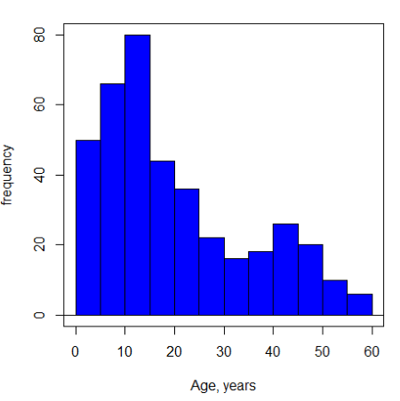
Figure 3. Histogram of ages of subjects in the diabetic retinopathy data set in the survival package.
Doesn’t look like a normal distribution, does it/?.
Z-score or Chebyshev’s inequality, which to use /? Chebyshev’s inequality is more general — it can be used whether the variables is discrete or continuous and without assumption about the distribution. In contrast, the Z score assumes more is known about the variable: random, continuous, drawn from a normally distributed population. Thus, as long as these assumptions hold, the Z score approach will give a better answer. Makes intuitive sense — if we know more, our predictions should be better.
In summary from the above points, and perhaps more formally for our purposes, the standard deviation is a good statistic to describe variability of observations on subjects, it’s integral to the concept of precision of an estimate and is part of any equation for calculating confidence intervals (CI). For any estimated statistic, a good rule of thumb is to always include a confidence interval calculation. We introduced these intervals in our discussion of risk analysis (approximate CI of NNT), and we will return to confidence intervals more formally when we introduce t-tests.
When you hear people talk about “margin of error” in a survey, typically they are referring to the standard deviation — to be more precise, they are referring to a calculation that includes the standard deviation, the standard error and an accounting for confidence in the estimate (see also Chapter 3.5 – Statistics of error).
Corrected Sums of Squares.
Now, take a closer look at the sample variance formula. We see a deviate

The variance is the average of the squared deviations from the mean. Because of the “squared” part, this statistic will always be positive and greater (or typically, equal to) zero. The variance has squared units (eg, if the units were grams, then the variance units are grams2). The sample standard deviation has the same units as the quantity (ie, no “squared” term). The numerator is called a sums of squares, and will be abbreviated as SS. Much like the deviate, will show up frequently as we move forward in statistics (eg, it’s key to understanding ANOVA).
Other standard deviations of means.
Just as we discussed for the arithmetic average, there will be corresponding standard deviations for the other kinds of means. With the geometric mean, one would calculate the standard deviation of the geometric mean, sgm, as
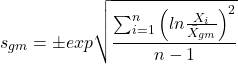
where exp is the exponential function, ln refers to natural logarithm, and  refers to the sample geometric mean.
For the sample harmonic mean, it turns out there isn’t a straight-forward formula, only an approximation (which I will spare you — it involves use of expectations and moments).
Base R, and therefore Rcmdr, doesn’t have built in functions for these, although you could download and install some R packages which do (eg, package NCStats, and the function is geosd() ).
If we run into data types appropriate for the geometric or harmonic means and standard deviations I will point these out; for now, I present these for completeness only.
Coefficient of variation (CV).
An unfortunate property of the standard deviation is that it is related (= “correlated”) to the mean — a fact recognized by Pearson (1896, p 276). Thus, if the mean of a sample of 100 individuals is 5 and variability is about 20%, then the standard deviation is about 1; compare to a sample of 100 individuals with mean = 25 and 20% variability, the standard deviation is about 5. For means ranging from 1 to 100, here’s a plot to show you what I am talking about.
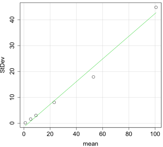
Figure 4. Scatter plot of the standard deviation (StDev) by the mean. Data sets were simulated.
The data presented in the Figure 4 graph were simulated. Is this bias, a correlation between mean and standard deviation, something you’d see in “real” data? Here’s a plot of height in inches at withers for dog breeds (Fig 5). A line is drawn (ordinary linear regression, see Chapter 17) and as you can see, as the mean increases, the variability as indicated by the standard deviation also increases.
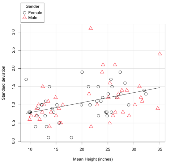
Figure 5. Plot of the standard deviation by the mean for heights of different breeds of dogs.
So, to compare variability estimates among groups when the means also vary, we need a new statistic, the coefficient of variation, abbreviated CV (Pearson 1896). The coefficient of variation is also known as the relative standard deviation, RSD. Many statistics textbooks not aimed at biologists do not provide this estimator (eg, check your statistics book).
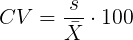
This is simply the standard deviation of the sample divided by the sample mean, then multiplied by 100 to give a percent. The CV is useful when comparing the distributions of different types of data with different means.
Many times, the standard deviation of a distribution will be associated with the mean of the data.
Example. The standard deviation in height of elephants will be larger on the centimeter scale than the standard deviation of the height of mice. However, the amount of variability RELATIVE to the mean may be similar between elephants and mice. The CV might indicate that the relative variability of the two organisms is the same.
The standard deviation will also be influenced by the scale of measurement. If you measure on the mm scale versus the meter scale the magnitude of the SD will change. However, the CV will be the same!
By dividing the standard deviation by the mean you remove the measurement scale dependence of the standard deviation and generally, you also remove the relationship of the standard deviation with the mean. Therefore, CV is useful when comparing the variability of the data from distributions with different means.
One disadvantage is that the CV is only useful for ratio scale data (ie, those with a true zero).
The coefficient of variation is also one of the statistics useful for describing the precision of a measurement. See Chapter 3.4 Estimating parameters.
Standard error of the mean (SEM).
All estimates should be accompanied by a statistic that describes the accuracy of the measure. Combined with the confidence interval (Chapter 3.4), one such statistic is called the standard error of the mean, or SEM for short. For the error associated with calculation of our sample mean, it is defined as the sample standard deviation divided by the square root of n, the sample size.
sem → 
The concept of error for estimates is a crucial concept. All estimates are made with error and for many statistics, a calculation is available to estimate the error (see Chapter 3.4).
Although related to each other, the concepts of sample standard deviation and sample standard error have distinct interpretations in statistics. The standard deviation quantifies the amount of variation of observations from the mean, while the standard error quantifies the difference between the sample mean and the population mean. The standard error will always be smaller than the standard deviation and is best left for reporting accuracy of a measure and statistical inference rather than description.
Questions.
- For a sample data set like
myY <- c(1,1,3,6), you should now be able to calculate, by hand, the
• range
• mean
• median
• mode
• standard deviation
• coefficient of variation - For our example data set,
myX <- c(4,4,4,4,5,6,6,6,7,7,8,8,8,8,8)calculate
• IQR
• sample standard deviation, s
• coefficient of variation - Use the
sample()command in R to draw samples of size 4, 8, and 12 from your example data set stored inmyX. Repeat the calculations from question 4. For examplex4 <- sample(x,4)will randomly select four observations from x, and will store it in the object x4, like so (your numbers probably will differ!)x4 <- sample(x,4); x4 [1] 8 6 8 6 - Repeat the exercise in question 4 again using different samples of 4, 8, and 12. For example, when I repeat sample(
x,4) a second time I getsample(x,4) [1] 8 4 8 6 - For Table 1, determine how many multiples of the standard deviation for observations greater than 95-percentile (eg, determine the observation value for a person who is in the 95-percentile for Height in the different decades, etc.
- Calculate the sample range, IQR, sample standard deviation, and coefficient of variation for the following data sets
• Height in inches of mothers,mom <- c(67, 66.5, 64, 58.5, 68, 66.5) #(data from GaltonFamilies in R package HistData)
and fathers,dad <- c(78.5, 75.5, 75, 75, 74, 74) #(data from GaltonFamilies in R package HistData)
• Carbon dioxide (CO2) readings from Mauna Loa for the month of December for
years <-c (1960, 1965, 1970, 1975, 1980, 1985, 1990, 1995, 2000, 2005, 2010, 2015, 2020)years <-c (1960, 1965, 1970, 1975, 1980, 1985, 1990, 1995, 2000, 2005, 2010, 2015, 2020) #obviously, do not calculate statistics on years; you can use to make a plotco2 <- c(316.19, 319.42, 325.13, 330.62, 338.29, 346.12, 354.41, 360.82, 396.83, 380.31, 389.99, 402.06, 414.26) #(data from Dr. Pieter Tans, NOAA/GML (gml.noaa.gov/ccgg/trends/) and Dr. Ralph Keeling, Scripps Institution of Oceanography (scrippsco2.ucsd.edu/))
• Body mass of Rhinella marina (formerly Bufo marinus) (see Fig. 1),bufo <- c(71.3, 71.4, 74.1, 85.4, 85.4, 86.6, 97.4, 99.6, 107, 115.7, 135.7, 156.2)
Quiz – Chapter 3.3
Measures of dispersion
Chapter 3 contents
2.6 – Statistical reasoning
How statistical reasoning helps us spot and reduce bias.
.
So far in the course we have talked about statistical reasoning. Statistical reasoning as part of the critical thinking tool kit. What this should mean for you in practice is that we will be developing and enhancing your critical thinking skill set. Here, we’ll define our terms and place statistical reasoning in context.
Critical thinking.
.
What do I mean by critical thinking? You’ll find various definitions and discussions, but the Wikipedia entry on the subject seems as good a start as anything else I have heard or read:
“Critical thinking is a way of deciding whether a claim is always true, sometimes true, partly true, or false” (5 August 2013, http://en.wikipedia.org/wiki/Critical_thinking).
Which raises the question, what is truth (false)? And what about the frequency qualifiers “always,” “sometimes,” “partly”? This hints at one of the strengths of science; “Truth in science … is never final, and what is accepted as fact today may be modified or even discarded tomorrow” (p. 2, National Academy of Science 1999). Scientists extend and even correct the work of their predecessors.
Critical thinking has many definitions, but they coalesce broadly as the search for rational justification — arguments and decisions based on reason not emotion — given sets of facts. We’ll define facts as assertions about the world that are verifiably true. Related to facts, we define evidence as collection of facts used to infer an assertion or belief is objectively true. Objectivity holds independently of the observer. In practice, critical thinking can be improved by identifying and developing certain skill sets, from deductive reasoning to use of a statistical toolkit, although skills alone do not necessarily lead to sound critical thinking (Bailin 2002). Emphasis on the importance of statistical reasoning, for example in the Evidence-Based Medicine (EBM) approach, is now well established. EBM is an expansive concept, but includes the philosophy that decisions in medicine and health care should be based on evidence (results) from well designed and executed research. More generally, much has been written on the subject. My purpose here is to sell you just a bit that you will learn more than formulas and statistical tests in this course; if we do this right you will improve your critical thinking skills.
And the tool kit for critical thinking? Science has the scientific method to offer. In turn, by adopting statistical reasoning approaches you will be more cognizant of whether or not you are indeed engaged in critical thinking about your work.
A working checklist for critical evaluation of a project
- “All sides” of the problem are fairly represented
- Authority is not synonymous with empirical truth: trust, but verify
- Correlation (association) may or may not infer causation
- Do conflicts of interest compromise conclusions?
In other words, identify and rigorously consider assumptions made to reach conclusions, evidence given in support of conclusions, and considerations of bias held by the researcher. The “all sides” part requires judgement — not all sides of a research question are equally valid; the point about “fair” representation requires that opposing arguments are actually held by others and not simply a “”straw man” characterization of of a position held by no one.
Rigid adherence to “how to do science checklist” is likely to be wanting and thus practicing and successful scientists show more flexibility. And, the list is certainly incomplete because it presumes observations and data collection are from a reliable, unbiased source. Before proceeding with how statistics informs our critical thinking in science, let’s illustrate bias.
Bias everywhere.
.
Bias is defined as any tendency that may hamper our ability to answer a question without prejudice (Pannucci and Wilkins 2010). Although we tend to think of ourselves as highly rational (Note 1), psychologists have documented, named numerous, and in some cases, highly specific kinds of cognitive biases we may have about “real world data” that may impair our judgment about results of experiments.
Note 1. A handful of Nobel prizes were awarded over evidence and theory on just how unrational we are, see Simon (1978), Kahneman (2002), and Thaler (2017, whose views were immortalized in the movie The Big Short).
At its best, application of the scientific method is our best tool kit to help protect our conclusions against bias (Nuzzo 2015), by proper experimental design and possible study biases. A couple of comics from xkcd illustrate.
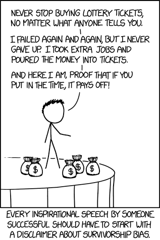
Figure 1. “Survivorship bias,” https://www.xkcd.com/1827/ .
Figure 2. “Selection bias,” https://xkcd.com/2618/ .
Wikipedia lists dozens of named biases which may influence our ability to interpret science:
- confirmation bias, eg, given extraneous information about ancestry or sex, forensic investigators were more likely to assign ancestry or sex of skeletal evidence to group that confirmed the contextual information (Nakhaeizadeh et al 2014).
- congruence bias, a type of confirmation bias, the tendency to test only a favorite or initial hypothesis over consideration of alternative hypotheses.
- observer-expectancy bias, eg, randomized controlled trials of acupuncture often find equivalent responses to real and placebo acupuncture despite both appearing superior to no treatment (Colagiuri and Smith 2012).
- selection bias, the selection of individuals, groups, or data for analysis in such a way that proper randomization is not achieved, eg, mitotic counts (Cree et al 2021) and cell differentials and Figure 2. Selection bias, where the study population is not well-defined or if is, the method by which subjects are recruited favors one kind of subject over another.
- surveillance bias, eg, association between myocarditis and COVID-19 vaccines may be due to increased focus to identify myocarditis (Husby et al 2021).
- survivorship bias, focusing on subjects that passed a selection process as if they represent an entire group, eg, from ecology: rare species more likely to go extinct than abundant species (Lockwood 2003) and Figure 1.
Bias in research may occur at any level, from study design to analysis and publication of results. Bias leads to systematic errors that may favor one outcome over others. Clearly then, bias is something one wants to avoid in science, and most scientists would probably agree strongly that bias is unacceptable. However, bias can creep into projects in many forms.
Particularly pernicious causes of bias are conflicts of interest, with the notable case of a 1990’s set of trials in gene therapy (Wilson 2010). Biased research may be more harmful to science than deliberate misconduct, at least in part because there are, or should be, mechanisms to detect fraud (eg, Marusic et al 2007). If errors in data analysis or management are rare, we can trust the results; if errors are common, systematic, or deliberate falsification, then any conclusions drawn from such work deserves retraction at the very least (cf. discussion in Baggerly and Coombs 2009; see StatCheck project, Nuijten et al 12016).
Bias in research.
.
Bias is not limited to obvious profit seeking or even defense of one’s ideas or reputation. Bias can enter research in subtle ways. Prior to 2000, many post-menopausal women could expect to be placed on hormone replacement therapy (HRT) to manage post-menopausal symptoms and to reduce likelihood of osteoporosis later in life. Moreover, HRT was believed based on research to show protective benefits against heart disease (eg, Nabulsi et al 1993; Grodstein et al 2000). However, other prospective studies that were designed to reduce many sources of bias in patient recruitment (Women’s Health Initiative Study Group 1998), found the opposite: HRT may increase risk of heart disease as well as other diseases (Rossouw et al 2002). Since the 2002 Women’s Health Initiative study report, the costs and benefits of HRT have been furiously debated (Lukes 2008).
The purpose of this chapter, however, is not to exhaustively review sources of bias. Instead, we leave you with a partial list of kinds of bias in clinical trials (from a review by Pannucci and Wilkins 2010).
- Bias during study design, eg, use of subjective measures or poorly designed questionnaires.
- Interviewer bias, for example, if the interviewer is aware of the subject’s condition
- Chronology bias, where the control subjects may not be observed in the same time frame as the treatment subjects
- Citation (reporting) bias, where negative results are not reported
- Confounding, where results may be due to factors not properly controlled that also affect the outcome. An example provided was link between income and health status, which would be confounded by access to health care.
These are but a few of the kinds of bias that even proper research may be influenced by. Solutions are to randomize, to double-blind, and to avoid reporting bias. Controls of sources of bias increase the validity of the research. How experimental design may control for bias is discussed further in Chapter 5.3.
A case study.
.
Stories we hear from the news or from our friends about health or the environment are anecdotal. A basic rule in critical thinking is to distinguish between argument that is built on anecdotal evidence and argument based on scientific evidence. Let’s evaluate the following real-world example.
Airborne® is a leading dietary supplement. Here’s what their website has to say about the product.
“Scientific research confirms that Airborne proprietary formulation with 13 vitamins and minerals plus a blend of health-promoting herbs, does indeed enhance immunity (5 August 2013, http://www.airbornehealth.com/our-story).
This next statement appears in smaller text near the bottom of the page.
“These statements have not been evaluated by the Food and Drug Administration. These products are not intended to diagnose, treat, cure or prevent disease” (5 August 2013, http://www.airbornehealth.com/our-story).
So, in short, how do you evaluate Airborne? The claim is that “scientific research confirms that Airborne … enhance immunity,” and yet, there is a statement that follows that suggests that the claim has not been evaluated by the agency legally responsible in the USA for determining the efficacy of medicine and treatments.
Note 2. “enhance” immunity is a vacuous phrase. Immunity is not a single object. If by immunity we mean resistant to a particular pathogen, this cannot be what the makers literally mean because that would be in violation of the FDA. Yes, deficiencies of vitamin C and other nutrients impair immune function (Carr and Maggini 2017), but there is no evidence to support the claim that Vitamin C supplementation above RDA, recommended dietary allowances, improves resistance. See 2013 Cochrane Review.
Are not these in contradiction? In the USA, supplement manufactures’ need not seek FDA approval. In fact, the U.S. Congress, in it’s passing of the The Dietary Supplement Health and Education Act of 1994 (DSHEA), specified what needs to be reported to the FDA; statements of “enhancing immunity” are lawful, but do not require the supplement manufacture to show evidence that their product provides this support, only that ingredients in the supplement may do so.
Returning to the statements from Airborne Health, how may these statements be interpreted?
- peer-reviewed articles testing Airborne are available
- that experiments were conducted without bias
- and that to “enhance immunity” is something one could measure
Let’s look at #3 first. A search of PubMed (December 2013) for the phrase “enhance immunity” returned 9171 hits. I didn’t look through the more than 9000 articles, but a quick look shows that the term is indeed used in research, but carries a wide range of interpretations. For one paper “enhance immune” response was the result of genetic modifications to T-cells and how they responded to a virus (PMID:24324159).
Adding “vitamin” to the search resulted in just 158 hits in PubMed; none of these are about Airborne (see claim #1 and #2). However, to be fair, go back and look at their statement — notice they are not saying exactly that anyone has studied Airborne (otherwise they’d probably list the papers), just that vitamins and minerals and herbs that are in Airborne have been studied.
Indeed, vitamins A, C, E and minerals like zinc and selenium that are in Airborne are among the 158 papers. To be additionally fair to Airborne, there are indeed many papers investigating benefits (harm) of supplemental vitamins and minerals — and again, being charitable here, what we can say is that results are at best inconsistent (Bjelakovic et al 2014; Comerford 2013).
The manufacturer of Airborne ran into some trouble with the FTC and ended up paying over $20 million US dollars to settle the lawsuit. The one study, not peer-reviewed, of Airborne’s effectiveness cited during these proceedings apparently was sponsored by Airborne’s manufacturer. Airborne was acquired by Schiff Vitamins March 2012 (Bloomberg News). Click here for additional reading about Airborne.
About peer-review.
.
Evaluation of claims made, research reported, and ideas in science are generally expected to be subject to peer-review by knowledgeable persons in the field. Effective peer-review is an important “gatekeeper” in science (Siler et al 2015, Tennant 2018). Proper peer review gives legitimacy to research (Siler et al 2015). The traditional peer review system is a closed system, which includes elements controlled by journal editors and is based on reviewer identify remaining anonymous. The closed peer-review system is not the only option: many have argued for an open review process (eg, Pöschl 2012, Ho et al 2013).
Does the Airborne story meet your definition of bias?
.
Airborne made health claims I about their product; these claims were found by the federal government to be misleading but does not fit into our discussion of bias. Instead, Airborne story fits more with critical thinking: I think it is rather a casual position to say that we should, and do, think critically of news source or the stories our friends tell us about health.
But bias in science occurs too, and can be very difficult to control or completely eliminate.
Learning statistical reasoning will help develop critical thinking skills.
.
In addition to considering sources of bias, ie, can you trust the messenger, thinking about the sets of facts offered to bolster a claim, it helps to evaluate each fact to see if
- The author is really talking about correlation and has not in fact provided evidence of causation
- vs. experiment, which tests “cause” manipulate
X, doesYchange?
- vs. experiment, which tests “cause” manipulate
- Measurement appropriate?
- Direct or indirect
- Unmeasured important (co)variable
Questions.
.
- Write up three learning outcomes for this page. Hint: Point your favorite generative AI to this page and ask for help.
- The xkcd comic in Figure 1 titles calls it survivorship bias. Provide a definition for this kind of bias and describe the effects on conclusions if it is not accounted for.
- Doctors are encouraged to engage in “evidence based medicine,” that is, decisions about care should be based on data. How may confirmatory bias (from the patient’s point of view, from the doctor’s point of view) influence a discussion of “facts” when deciding on a course of medication therapy — between a well-established medication with many known side-effects and a new, recently approved medicine reported to be as effective as the standard treatment.
Quiz Chapter 2.6
Statistical reasoning
Chapter 2 contents
.
2.4 – Experimental Design and rise of statistics in medical research
Experiments and observations: Finding answers.
.
How to identify cause and effect, and the kinds of evidence that can be inferred from the various approaches to study causes of disease has became a major source of disagreement in the news. In a fascinating study, Pew Research Center reported “half of U.S. adults under 50 say they get health and wellness information from social media influencers or podcasts,” and, only about 17% of these influencers report “conventional medicine” training (Report, May 7 2026). For our purposes, I made substantial updates to this page in the fifth month after WHO had declared the Covid-19 pandemic (CDC timeline), and continue to do so today.
The pandemic left many life-lessons, for scientists and public-health supporters, but also for everyone who lived through those times. One of the lessons was how to deal with the challenges of finding treatments in real time. If you followed the news early in the pandemic, you know of the appeal from some (including Donald Trump, the then-President of the United States, Boseley 2020), for use of an anti-parasite drug, hydroxychloroquine, as prophylactic or treatment for active Covid-19 infection (cf. Liu et al 2020). The FDA as well as other institutions rapidly advised against use, in part because experimental design concerns were raised for early studies (Kupferschmidt, 2020). The issue remains contentious for some (eg, Health and Human Services Secretary Robert F. Kennedy Jr., CNN August 2, 2026 interview).
Thus, job number one for students of biostatistics is to learn how to weigh arguments for or against therapies or treatments offered. The purpose of this page is to introduce these issues — how to judge whether a treatment is effective or not.
We will spend some time later on statistical aspects of experimental design (Chapter 5), but we begin with Randomized Control Trials, or RCT, as a model for our discussion of experimental studies. The RCT we recognize today owes its beginning to the 1948 studies on streptomycin use to treat tuberculosis (British Medical Research Council 1948), but of course, the foundations of RCT and experimental design in general, go back much earlier than that date (Chalmers 2011, Hairton and Locascio 2018). For a number of reasons the RCT — experimental, prospective, double-blind clinical trial with random selection of subjects from a reference population and random assignment of subjects to a treatment group or an appropriate placebo treatment control group — is considered the “gold standard” method for producing knowledge (Kaptchuk 2001, Hairton and Locascio 2018).
Note 1. I use the phrase “gold standard” associated with the RCT in the historical context intended by the authors cited. Unfortunately, in 2025, the phrase “gold standard science” has become political (Lewandowsky 2025, Mervis 2025). What we can agree on is characteristics of research as good science: “reproducible; transparent; communicative of error and uncertainty; collaborative and interdisciplinary; skeptical of its findings and assumptions; structured for falsifiability of hypotheses; subject to unbiased peer review; accepting of negative results as positive outcomes; and without conflicts of interest,” Sec. 3. Restoring Gold Standard Science, Presidential Executive Order, May 23, 2025. But even this list is not above scrutiny.
This discourse is way above my pay grade, but for starters, I would replace “without conflicts of interest” with “without disclosure of potential conflicts of interest.” The latter is practical, the former is likely not at all achievable. After all, even where a conflict exists, it does not immediately follow that the reported science is bad, that the conflict is evidence by itself of bias. Reporting conflicts warns the reader that results and conclusions may warrant further scrutiny, but outright dismissal is itself contrary to good science practice. Certainly, there are other aspects to defining what is and what is not good science. And, “gold standard” is just a metaphor (Love 2003), and, frankly, a very out-dated one. The United States and most other nations long ago gave up — for many good reasons — the gold standard as a monetary standard.
Technically, RCT are intervention trials, a specific application of the more general definition of an experiment. That is, the researchers tests a potential drug or therapy in people to observe its effect while holding other variables constant. Experimental studies imply that the researcher imposed treatments or controls onto subjects. The subjects are followed and outcomes are recorded. Thus, experiments by definition are also prospective studies — the outcome is recorded for subjects after some period of time. With a well-designed experiment, the researcher may have evidence to support the claim that, for example, Treatment A causes the outcome.
RCT applied to human health can have profound impact on lives.
The ALLHAT-LLT (JAMA, 2002) trial tested whether adding the cholesterol-lowering drug pravastatin to standard care would reduce heart attacks and deaths in people with high blood pressure and moderately high cholesterol. The study found no significant benefit compared to usual care, suggesting that statin therapy may not always provide extra protection in this group. Its results helped refine how doctors balance blood pressure and cholesterol treatment in heart disease prevention.
The Women’s Health Initiative (JAMA, 2002) trial tested the effects of combined estrogen and progestin therapy in healthy postmenopausal women. It found that while the therapy slightly reduced the risk of fractures and colon cancer, it increased the risk of heart disease, stroke, and breast cancer. These results transformed medical guidance by showing that hormone therapy should not be routinely used to prevent chronic disease in postmenopausal women.
The Du Toit et al. (NEJM, 2015) study showed that introducing peanut-containing foods early in life — rather than avoiding them — greatly reduced the risk of developing peanut allergies in high-risk infants. This landmark randomized trial changed how doctors think about food allergies, leading to new guidelines that encourage early introduction instead of avoidance.
And more recently, we have study reported by Deanfield et al (Lancet, 2025), which found that semaglutide reduced the risk of major adverse cardiovascular events (MACE) in adults with overweight or obesity and established cardiovascular disease—even if they did not lose much weight or had lower baseline adiposity.
In contrast, observational studies are those in which treatments arise by acts of nature. In both experiments and observational studies, there can be treatment and control groups; the distinction between the types of studies is how assignment of subjects to treatments were affected. Observational studies generally are retrospective studies — the outcome has already occurred, the researcher follows up to identify differences among the groups that may account for different outcomes. Examples of observational, retrospective study designs include cross-sectional and case control; cohort studies are prospective studies. Observational studies are discussed further in Chapter 5.4 – Clinical trials.
Compared to observational studies, in principle, experiments can establish cause and effect. Cause and effect refers to an explanation about relationship between two events or objects. In biology, Ernst Mayr (1904 – 2005) distinguished between two levels of explanation, proximate (how) explanations and ultimate (why) explanations (Mayr 1961, cf. Laland et al. 2011). As you know, our mechanism for identifying cause and effect is application of the Scientific Method (Chapter 2.5). Discussions of how to detect cause and effect are provided throughout this book, but emphasized in a few sections (Chapter 16.2 and 16.3).
Good experiments.
The principles of good experiments include many steps beyond simply choosing treatments and controls. In Chapter 5 we’ll go into more depth, but I wished to list for you some of the key principles of good experimental design. With respect to human-subject research, the researcher needs to protect against many sources of potential bias.
- Randomization of subjects assigned to treatment groups controls for individual differences.
- Controls (eg, Placebos) are a means to establish controls in a study so that effects may be attributed to the active treatment.
- Single-blind implies that the subject does not know what treatment was given.
- Double-blind implies that not only is the subject unaware of the treatment received, but, crucially, neither does the researcher.
- The double-blind design — neither the patient-subject nor the researchers know who received the placebo or the treatment — controls for subtle biases.
Note 2. Experimental control implies researcher imposes conditions to remove possibly confounding effects on the dependent variable — outcome of the experiment. Placebo, derived from Latin placere, to please (but see Aronson 1999). Placebo refers to an inert substance (“sugar pill”), or to a substance with known activity but without effect on the target condition or “wrong indication” (eg, antibiotics administered for viral infection), given to research subjects in lieu of the active treatment of interest (the hypothesis). Thus, placebos are examples of treatment controls.
The placebo effect is improvement of subjects who received the placebo and not active treatment (Pardo-Cabello et al 2022). In contrast, nocebo effects are adverse effects attributed to placebo treatment. Under most circumstances, placebo applies to humans only because placebo effects are thought to be product of psychological factors, although mechanisms of action are in dispute. Is sentience necessary for a placebo effect (cf. McMillan 1999)?
The experimenter may influence the outcome of the experiment if knowledge about who received the placebo or the new drug; the subject may respond differently with knowledge that they received the placebo and not the new drug. The key intent in this experimental design is to avoid systematic error, errors in studies that may occur because of our conscious and unconscious beliefs and biases. Placebos are used as treatments because people (and animals!) sometimes get better (or worse) with or without treatment; thus, to be effective, subjects receiving a new drug must get better more frequently than do subjects on placebo. Importantly, the well-designed placebo allows the researcher to gain insight into the mechanism of action by the new drug.
A case to consider: Comparing migraine treatments.
.
Consider the following experiment (Diener et al 2006; see also Liu et al 2018): subjects who had several migraines per month were treated with acupuncture, sham-acupuncture, or standard treatments including beta blockers, calcium channel blockers, or antiepileptic drugs. After 26 weeks the reductions in reported migraines was compared. The authors reported that there was no difference in numbers of migraines among patients who received the different therapy treatments. The authors conclude that because acupuncture lacks side-effects that may occur with standard therapies acupuncture may be a good choice for patients seeking relief from migraine. This is a classic experiment — subjects were assigned to treatments by the researchers. At least in principle, if one treatment group showed better outcomes, the improvement could be attributed to the treatment.
Another case to consider: When the cause isn’t clear.
.
Consider the following example. My dad was diagnosed with lung cancer in his late 70s; his left lung showed many spots when imaged and biopsy confirmed. Surgeons removed half of the lung and after several years he was considered cancer free. Why did he develop cancer in the first place? If you immediately think, “He’s a smoker,” that’s not a good explanation — and shame on you, you’re first instinct was to blame the patient (see discussion in Huff 2013). Dad last smoked tobacco in his early thirties (latency smoking-lung cancer link about 20 years, Lipfert et al 2019).
Tobacco smoking is not the only environmental trigger for lung cancer. Cancer of the lung in non-smokers is the seventh leading cause of cancer mortality worldwide (Field and Withers 2012). Long term exposure to radon gas, a naturally occurring, radioactive noble gas has been linked to lung cancer (EPA). I grew up on Vashon Island, Washington, in a non-smoking home environment. Radon levels on Vashon Island and other areas around Puget Sound are low (source: Washington State Department of Health). Radon is out as an explanation.
What other environmental sources may be linked to cancer? Vashon Island is rural, but, as it turned out, within range of effluent from a copper smelter located in nearby Ruston, Pierce County (Fig 1; my home was 17 km distance from the smelter).

Figure 1. Left: ASARCO smelter, Ruston, Washington, image from Department of Ecology, State of Washington. Direction of smoke from the stack is north, toward Vashon Island. Right: Voronoi map of arsenic and lead affected areas. image from kingcounty.gov. Darker regions correspond to heavier arsenic and lead contamination of soils.
The smelter was last in operation in 1986 and was torn down in 1993 (EPA publication number 910R94001). The smelter stack rose more than 500 feet dispersing smoke laden with heavy metals, notably inorganic arsenic and lead, into the air (Bromenshenk et al. 1985). Over the smelter’s 68 years of service, winds carried away the smoke to my island and to other areas known now as the “Ruston-Vashon Island Exposure Pathway” (Kalman et al 1990). The former smelter site was among the first listed Superfund sites (1983) in the United States by the EPA. Thus, tens of thousands of people were (and continue to be) exposed to the heavy metals deposited into the soils, forming a distinct exposure group (Milham & Strong 1974; Kalman et al 1990; EPA 2000). Arsenic exposure can be via inhalation, skin, or in drinking water — areas of Vashon-Maury island continue to have high levels of arsenic in both the soil and in any domestic water wells (PublicationNo. 14-09-044, Department of Ecology State of Washington).
Note 3: A personal comment — I stumbled onto the article by Bromenshenk and colleagues by accident. Instead of attending lecture, as I often did at the time, I was looking through journals in the research library. I was shocked at this article, because for the first time, I connected the smelter to the island I grew up on. The contamination on the island just wasn’t a conversation.
Is arsenic exposure by inhalation a plausible mechanism for my Dad’s lung cancer? As shown in Fig 1, the soils on Vashon near my home were heavily impacted by the smelter. Exposure could have come about from exposure during routine yard work — I have memories of clouds of dust kicked up by the lawn mower during spring and summers. Thus, an exposure route is possible. What evidence can we come up with?
Figure 2A shows negative association between lung and bronchial cancer incidence rates per 100L persons, adjusted for age, for several Washington state counties between 2000 and 2020 and distance from the smelter in Ruston. For comparison, Figure 2B shows no association between bladder cancer incidence rates per 100K for the same counties and time period and distance from the smelter. Workers exposed to arsenic have higher rates of lung cancer (Sullivan 2007, Wei et al 2019; see Enterline et al 1987 for a study a study based on cancer of workers at the smelter). Cultured lung cells exposed to arsenic associated with changes in gene expression (Clancy et al 2012). Coincidently, two of the family dogs developed and died of cancer as did one female goat. Perhaps my dad’s lung cancer was attributed to long exposure to arsenic (a decade after the cancer, and long after he stopped with yard work, his blood readings for arsenic were in the range of a modest 11 μg/L).
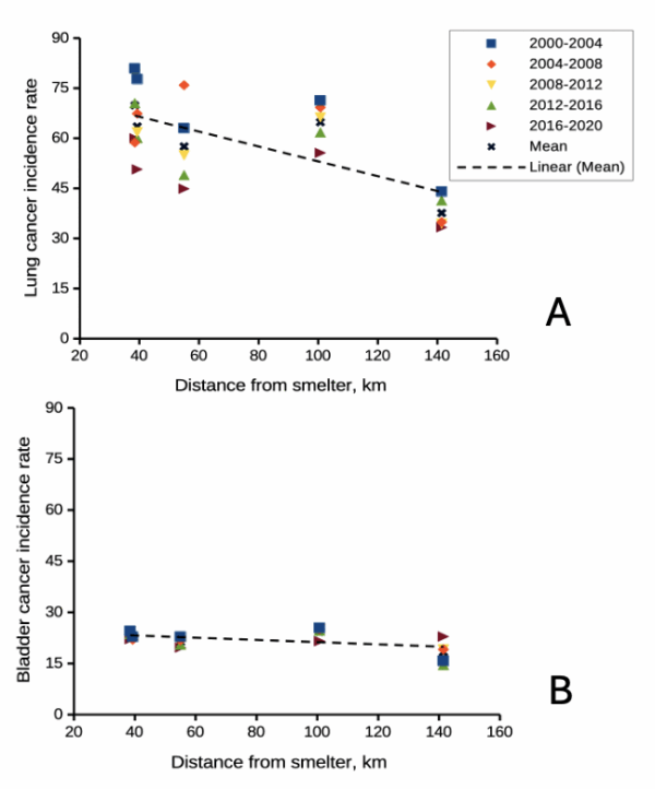
Figure 2. County cancer rates (A, lung and bronchial; B, bladder) from 2000 – 2020 vs distance in kilometers from ASARCO smelter, Ruston, WA. Data compiled from Washington Tracking Network (WTN). The counties were King (55 km), Kitsap (39.28 km), Pierce (38.48 km), San Juan ( 141.43 km), Snohomish (100.73 km), and Spokane (385.34 km).
If this scenario seems plausible, I hope you immediately recognize it as a case of confirmation bias (see Chapter 2.6). Putting aside for a moment the different arsenic species, each with different LD50 (the lethal dose needed to kill half the population — see Chapter 20.10), the difficulty ascribing arsenic as a causal agent for my Dad’s cancer is that many other exposures happened simultaneously. For example, indoor carpets are a primary source of several volatile organic compounds (Haines et al 2020). Prior to 1980 carpets may have included formaldehyde and other known carcinogenic agents. Dad commuted by car between work and home — with a ferry ride between — for decades (until the early 1990s), routinely traveling heavily congested roadways, this during the years prior to and the early years of the Clean Air Act of Environmental Protection Agency of the United States (it wasn’t until 1981 that new cars met EPA emission standards: Clean Air Act timeline here). Thus, all commuters including my Dad were exposed to gasoline combustion emissions, many known to be carcinogenic (Parent et al 2007). Moreover, a limited study by Public Health of Seattle and King County (2001) found rates of cancer on Vashon between 1980 and 1988 were similar to other areas in King County.
Summary.
It’s easy to fall into the trap that experiments — and by extension meta-analysis and systematic reviews — are the best tools offered by science for developing knowledge about the world, and other approaches suffer by comparison. But after even a bit of reflection, we should recognize that it can’t be that simple. While we now “know” tobacco cigarette smoking increases lung cancer risk, and many experiments with animal models convincingly show the link (eg, Hutt et al 2005), no human experiment in the strict sense, ie, prospective, randomized control trial, has ever been conducted (hint: it would be unethical, see discussion in Allmark and Tod 2016). Instead, the accumulated evidence from observational studies on exposures of different populations over the years overwhelmingly points to smoking as a leading risk factor (cause) of lung and other cancers — an example of Hill’s guidelines of causality. We end with a quote:
RCTs can play a role in building scientific knowledge and useful predictions but they can only do so as part of a cumulative program, combining with other methods, including conceptual and theoretical development, to discover not ‘what works’, but ‘why things work’ (p 2, Deaton and Cartwright 2017).
Questions.
.
- Write up three learning outcomes for this page. Hint: Point your favorite generative AI to this page and ask for help.
- Was my Dad’s lung cancer attributable to his 40 years plus exposure to soil arsenic (he’s a non-smoker)? How should we approach this question?
- In Diener et al (2006), the authors concluded that because acupuncture lacks side-effects that may occur with standard therapies acupuncture may be a good choice for patients seeking relief from migraine. Do you agree with the authors?
- Ethical standards evolve with time. An ongoing debate in research is whether and how placebos are to be used in human subjects research. Placebos are a means to establish controls in a study so that effects may be attributed to the active treatment. The “gold standard” of clinical trials is considered to be the randomized double-blind design — neither the patient-subject nor the researchers know who receives the placebo or the treatment. Following review of the WHO report on Use of Placebos in Vaccine Trials, pick one study and evaluate whether or not the decision to use placebos was warranted in your opinion.
- I searched PUBMED for “double-blind” by decade and found the following results (August 2018) (Table 1). Open R and/or R Commander and create two variables, then generate a scatter plot. Describe the shape of the relationship between number of publications citing “double-blind” and time (eg, 1950 – 1959, 1960 – 1969, and so on).
| Decade | Publications |
|---|---|
| 1950 | 60 |
| 1960 | 995 |
| 1970 | 7184 |
| 1980 | 24737 |
| 1990 | 39643 |
| 2000 | 53965 |
| 2010 | 69265 |
- Here’s one way to enter this data into R. At the R prompt (or in the R Script window of R Commander), create two variables,
DecadeandPubsDecade <- c(seq(1950, 2020, by=10))Pubs <- c(59,995,7161,24728,39670,54011,57043)Make an XY scatter plotplot(Decade,Pubs) - Repeat the PUBMED search as above but search for “placebo”. Make a table like the one above and provide a scatterplot of your results.
- Is the concept of a placebo relevant if the subjects in your experiment are yeast cells, not humans?
- Similarly, if your subjects are yeast cells, how does the concept of performing experiments “blind” apply?
- Ethical standards change with time. An ongoing debate in research is whether and how placebos are to be used in human subjects research.
- If placebos are so important, why is their use a concern in clinical trials?
- Following review of the WHO report on Use of Placebos in Vaccine Trials (see Readings below), pick one study and evaluate whether or not the decision to use placebos was warranted in your opinion.
R notes for question 5:
<-is an assignment operator (assignOP); everything to the right of<-is assigned to the object named to the left of the<-operator. You can instead use=in place of<-, but because=is also used in other contexts besides assignment, a quick look at blogs by data scientists will find a preference to use<-for clarity and consistency.c()“combines” arguments into a vector.seq()is used to generate a sequence of numbers between a lower and an upper limit; ifby = nis included, the sequence will be increased by the value n. If omitted, then the sequence is increased by 1.
Quiz Chapter 2.4
Chapter 2 contents.
.
- Introduction
- Why biostatistics?
- Why do we use R Software?
- A brief history of (bio)statistics
- Experimental Design and rise of statistics in medical research
- Scientific method and where statistics fits
- Statistical reasoning
- Chapter 2 – References and suggested reading