3.5 – Statistics of error
Making sense of error in data.
This page explains how statistics of error help quantify differences between measured and true values, beginning with classical methods like standard error and confidence intervals that rely on large-sample assumptions. Related, statisticians talk about uncertainty — the quantification of doubt about a measurement. We introduce permutation-based approaches, including jackknife and bootstrap resampling, which avoid those assumptions and are especially useful with smaller or complex data sets. Observer variation (intra- and interobserver error) is also highlighted as an important source of measurement error.
Missing values are another common source of uncertainty in biological data sets. Data may be missing because of equipment failure, recording mistakes, sample loss, or biological factors that prevent a measurement from being collected. Even a small number of missing observations can influence summaries, graphs, and statistical tests, especially in smaller studies. In this chapter, we treat missing values mainly as a practical issue to identify and report during exploratory data analysis. Later, in the chapter on experimental design, we examine missing data in greater depth, including differences between random and non-random missingness, as well as approaches such as data imputation and the consequences these choices may have for interpretation.
We conclude with a discussion about confidence intervals as a measure of accuracy and emphasize proper use of significant figures to avoid overstating precision.
Statistics of error.
In statistics, error doesn’t mean mistake, an avoidable human misjudgement or oversight, eg, a typo. An error in statistics means there was a difference between the measured value and the actual value for an object. Efforts by many authors of notable classical statistics developed a large body of calculated statistics, eg, standard error the mean, which allows the user to quantify how large the error of measurement is given assumptions about the distribution of the errors. Thus, classical statistics requires user to make assumptions about the error distribution, the subject of our Chapter 6. A critical issue to understand is that these methods assume large sample sizes are available; they are called asymptotic statistics or large-sample statistics; the properties of the statistical estimates are evaluated as sample size approaches infinity.
Jackknife sampling and bootstrap sampling are permutation approaches to working with data when the Central Limit Theorem — as sample size increases, the distribution of sample means will tend to a normal distribution (see Chapter 6.7) — is unlikely to apply or, rather, we don’t wish to make that assumption (Chapter 19). The jackknife is a sampling method involving repeatedly sampling from the original data set, but each time leaving one value out. The estimator, for example, the sample mean, is calculated for each sample. The repeated estimates from the jackknife approach yield many estimates which, collected, are used to calculate the sample variance. Jackknife estimators tend to be less biased than those from classical asymptotic statistics.
Bootstrapping, and not jackknife resampling, may now be the preferred permutation approach (eg, Google Scholar search “bootstrap statistics” 36K hits; “jackknife statistics” 17K hits), but which method is best depends on qualities of the data set. Bootstrapping involves large numbers of permutations of the original data, which, in short, means we repeatedly take many samples of our data and recalculate our statistics on these sets of sampled data. We obtain statistical significance by comparing our result from the original data against how often results from our permutations on the resampled data sets exceed the originally observed results. By permutation methods, the goal is to avoid the assumptions made by large-sample statistical inference, ie, reaching conclusions about the population based on samples from the population. Since its introduction, “bootstrapping” has been shown to be superior in many — but, importantly, not all — cases for statistics of error compared to the standard, classical approach (Efron 1979, Hesterberg 2015).
There are many advocates for the permutation approaches, and, because we have computers now instead of the hand calculators our statistics ancestors used, permutation methods may be the approach you will take in your own work. However, the classical approach has its strengths — when the conditions, that is, when the assumptions of asymptotic statistics are met by the data, then the classical approaches tend to be less conservative than the permutation methods. By conservative, statisticians mean that a test performs at the level we expect it to. Thus, if the assumptions of classical statistics are met they return the correct answer more often than do the permutation tests.
Error and the observer.
Individual researchers make observations, therefore, we can talk about observer variation as a kind of error measurement. For repeated measures of the same object by an individual, we would expect the individual to return the same results. To the extent repeated measures differ, this is intraobserver error. In contrast, measures of the same object from different individuals is interobserver error. For a new instrument or measurement system, one would need to establish the reliability of the measure: confronted with the same object do researchers get the same measurement? Accounting for interobserver error applies in many fields, eg, histopathology of putative carcinoma slides (Franc et al 2003), liver biopsies for cirrhosis (Rousselet et al 2005), blood cell counts (Bacus 1973).
Confidence in estimates.
A really useful concept in statistics is the idea that you can assign how confident you are to an estimate. This is another way to speak of the accuracy of an estimate. Clearly, we have more confidence in a sample estimate for a population parameter if many observations are made. Another factor in our ability to estimate is the magnitude of observation differences. In general, the larger the differences among values from repeated trials, the less confident we will be in out estimate, unless, again, we make our estimates from a large collection of observations. These two quantities, sample size and variability, along with our level of confidence, eg, 95%, are incorporated into a statistic called the confidence interval.

We will use this concept a lot throughout the course; for now, a simple but approximate confidence interval is to use the 2 x SEM rule (as long as sample size large): twice the standard error of the mean. Take your estimate of the mean, then add (upper limit) or subtract (lower limit) twice the value of the standard error of the mean (if you recall, that’s the standard deviation divided by the square-root of the sample size).
Example. Consider five magnetic darts thrown at a dart board (28 cm diameter, height of 1.68m from the floor) from a distance of 3.15 meters (Fig 1).

Figure 1. Magnetic dart board with 5 darts. Click image to view full sized image.
The distance in centimeters (cm) between where each of the five darts landed on the board compared to the bullseye is reported in (Table 1),
Table 1. Results of five darts thrown at a target (Figure 2)*
| Dart | Distance |
|---|---|
| 1 | 7.5 |
| 2 | 3.0 |
| 3 | 1.0 |
| 4 | 2.7 |
| 5 | 7.4 |
* distance in centimeters from the center.
Note 1: Use of the coordinate plane, and including the angle measurement in addition to distance (the vector) from center, would be a better analysis. In the context of darts, determining accuracy of a thrower is an Aim-Point targeting problem and part of your calculation would be to get MOA (minute of angle). For the record, the angles (degrees) were
| Dart | Distance | Angle |
|---|---|---|
| 1 | 7.5 | 124.4 |
| 2 | 3.0 | -123.7 |
| 3 | 1.0 | 96.3 |
| 4 | 2.7 | -84.3 |
| 5 | 7.4 | -31.5 |
measured using imageJ. Because there seems to be an R package for just about every data analysis scenario, unsurprisingly, there’s an R package called shotGroups to analyze shooting data.
How precise was the dart thrower? We’ll use the coefficient of variation as a measure of precision. Second, how accurate were the throws? Use R to calculate
darts = c(7.5, 3.0, 1.0, 2.7, 7.4)
#use the coefficient of variation to describe precision of the throws
coefVar = 100*(sd(darts)/mean(darts)); coefVar
[1] 68.46141
Confidence Interval to describe accuracy.
For a game of darts, the true value would be a distance of zero — all bullseyes. We need to calculate the standard error of the mean (SEM), then, we calculate the confidence interval around the sample mean.
#Calculate the SEM
SEM <- sd(darts)/sqrt(length(darts)); SEM
[1] 1.322649
#now, get the lower and upper limit, subtract from the mean
confidence <- c(mean(darts)-2*SEM, mean(darts), mean(darts)+2*SEM); confidence
[1] 1.674702, 4.320000, 6.965298
The mean was 4.3 cm, therefore to get the lower limit of the interval subtract 2.65 (2*SEM = 2.645298) from the mean; for the upper limit add 2.65 to the mean. Thus, we report our approximate confidence interval as (1.7, 7.0), and we read this as saying we are about 95% confident the population value is between these two limits. Five is a very small sample number, so we shouldn’t be surprised to learn that our approximate confidence interval would be less than adequate. In statistical terms, we would use the t-distribution, and not the normal distribution, to make our confidence interval in cases like this.
Note 2: As a rule, implied by Central Limit theory and use of asymptotic statistical estimation, a sample size of 30 or more is safer, but probably unrealistic for many experiments. This is sometimes called as the rule of thirty. (For example, a 96-well PCR array costs about $500; with n = 30, that’s $15,000 US Dollars for one group!). So, what about this rule? This type of thinking should be avoided as “a relic of the pre-computer era,” (Hesterberg, T. (2008). It’s Time To Retire the” n>= 30″ rule.). We can improve on asymptotic statistics by applying bootstrap principles (Chapter 19).
We made a quick calculation of the confidence interval; we can get make this calculation by hand by incorporating the t distribution. We need to know the degrees of freedom, which in this case is 4 (n – 1, where n = 5). We look up critical value of t at 5% (to get our 95% confidence interval), t = 2.78. Subtract for lower limit t*SEM and add for upper limit t*SEM to the sample mean for the 95% confidence interval.
We can get help from R, by using the one-sample t-test with a test against the hypothesis that the true mean is equal to zero. Among a variety of output we will introduce later (see Chapter 8 and 10), the confidence interval is reported (yellow highlight),
#make an attach a data frame object
Ddarts <- data.frame(darts)
t.test(darts,mu=0)
One Sample t-test
data: darts
t = 3.2662, df = 4, p-value = 0.0309
alternative hypothesis: true mean is not equal to 0
95 percent confidence interval:
 0.6477381 7.9922619
sample estimates:
mean of x
 4.32
t.test uses the function qt(), which provides the quantile function. To recreate the 95% CI without the additional baggage output from the t.test, we would simply write
#upper limit
mean(darts)+ qt(0.975,df=4)*sd(darts)/sqrt(5)

#lower limit
mean(darts)+ qt(0.025, df = 4, lower.tail=TRUE)*sd(darts)/sqrt(5)
where sd(darts)/sqrt(5) is the standard error of the mean.
Or, alternatively, download and take advantage of a small package called Rmisc (not to be confused with the RcmdrMisc package) and use the function CI
library(Rmisc)
CI(darts)
     upper     mean     lower
7.9922619 4.3200000 0.6477381
The advantage of using the CI() command from the package Rmisc is pretty clear; I don’t have to specify the degrees of freedom or the standard error of the mean. By default, CI reports the 95% confidence interval. we can specify any interval simply by adding to the command. For example,
CI(darts, ci=0.90)
reports upper and lower limits for the 90% confidence interval.
Try it. On your own, get the 90% confidence interval and the 99% confidence intervals for our dart example. Compare to the 95% confidence interval — what do you conclude about “confidence” in our estimate from 90% to 99%?
Confidence intervals from p-values.
And finally, it is not unusual for a report to provide summary statistics, differences between means (ie, effect size), and p-values (orange highlight), but not report confidence intervals. We discuss p-values and the concept of statistical significance beginning in Chapter 8. But for now, we show how to calculate approximate confidence intervals from the p-value. This may be of use for conducting meta-analysis (Chapter 20.15). See two helpful “how to” articles by Bland and Altman in 2011 BMJ (references listed in Chapter 3.6 – References).
In brief, calculate the test statistic for a normal distribution (letZ), calculate a standard error, and then the lower and upper limits for the 95% confidence interval. We illustrate use of the calculator formulas with the dart example, the p-value was 0.0309; the estimate was 4.32.
R code
letZ = (-0.862 + sqrt(0.743 - 2.404*log(0.0309, base = exp(1)))) = 2.154903
letSE = 4.32/letZ = 2.00473
1.96*letSE = 3.929271 # Add for upper and subtract for lower
The lower limit is 0.39 (4.32 – 3.929271) and the upper limit is 8.25 (4.32 + 3.929271). Although in the ballpark, these calculated estimates are wider than the confidence interval estimated by the t.test command. Small sample size, n = 5, is to blame — the accuracy of these methods, based on asymptotic statistical estimation approaches, assumes the law of large numbers applies.
Significant figures.
And finally, we should respect significant figures, the number of digits which have meaning. Our data were measured to the nearest tenth of a centimeter, or two significant figures. Therefore, if we report the confidence interval as (0.6477381, 7.9922619), then we imply a false level of precision, unless we also report our random sampling error of measurement.
R has a number of ways to manage output. One option would be to set number of figures globally with the options() function — all values reported by R would hold for the entire session. For example, options(digits=3) would report all numbers to three significant figures. Instead, I prefer to use signif() function, which allows us to report just the values we wish and does not change reporting behavior for the entire session.
signif(CI(darts),2)
upper  mean lower
 8.00  4.30  0.65
Note 3: The options() function allows the R user to set a number of settings for an R session. After gaining familiarity with R, the advanced user recognizes that many settings can be changed to make the session work to report in ways more convenient to the user. If curious, submit options() at the R prompt and available settings will be displayed.
The R function signif() applies rounding rules. We apply rounding rules when required to report estimates to appropriate levels of precision. Rounding procedures are used to replace a number with a simplified approximation. Wikipedia provides a comprehensive list of rounding rules. Notable rules include
- directed rounding to an integer, eg, rounding up or down
- rounding to nearest integer, eg, round half up (down) if the number ends with 5
- randomly rounding to an integer, eg, stochastic rounding.
With the exception of stochastic rounding, all rounding methods impose biases on the sets of numbers. For example, the round half up method applied for numbers above 5, round down for numbers below 5 will increase the variance of the sample. In R, use round() for most of your work. If you need one of the other approaches, for example, to round up, the command is ceiling(); to round down we use floor().
When to round?
No doubt your previous math classes have cautioned you about the problems of rounding error and their influence on calculation. So, as a reminder, if reporting calls for rounding, then always round after you’ve completed your calculations, never during the calculations themselves.
A final note about significant figures and rounding. While the recommendations about reporting statistics are easy to come by (and often very proscriptive, eg, Table 1, Cole 2015), there are other concerns. Meta-analysis, which are done by collecting information from multiple studies, would benefit if more and not fewer numbers are reported, for the very same reason that we don’t round during calculations.
Questions
- Calculate the correct 90% and 99% confidence intervals for the dart data using the t-distribution
- by hand
- by one alternative method in R, demonstrated with examples in this page
- How many significant figures should be used for the volumetric pipettor p1000? The p200? The p20 (data at end of this page)?
- Another function,
round(), can be used. Try
round(CI(darts),2)
-
- and report the results: vary the significant figures from 1 to 10 (
signif()will take digits up to 22). - See any output differences between
signif()andround()? Don’t forget to take advantage of R help pages (eg, enter?roundat the R prompt) and see Wikipedia.
- and report the results: vary the significant figures from 1 to 10 (
- Compare rounding by
signif()andround()for the number 0.12345. Can you tell which rounding method the two functions use? - Calculate the coefficient of variation (CV) for each of the three volumetric pipettors from the data at end of this page. Rank the CV from smallest to largest. Which pipettor had the smallest CV and would therefore be judged the most precise?
- (data provided at end of this page, click here).
- Standards distinguish between within run precision and between run precision of a measurement instrument (see Chapter 16.5 – Instrument reliability and validity). The data in Table 1 were all recorded within 15 minutes by one operator. What kind pf precision was measured?
- Calculate the standard error of the means for each of the three pipettors from the data
- (data provided at end of this page, click here).
- Calculate the approximate confidence interval using the 2SE rule and judge which of the three pipettors is the most accurate (narrowest confidence interval)
- Repeat, but this time apply your preferred R method for obtaining confidence intervals.
- Compare approximate and R method confidence intervals. How well did the approximate method work?
- Return to the dart example, but now assume the p-value was p = 0.003 and again for p = 0.0003. Estimate the 95% confidence interval for each case; the difference remains 4.32. How does the change in p-value, from 0.03 to 0.0003 — a two orders of magnitude difference — affect the estimates for the confidence interval (hint: describe the width of the CI)?
Quiz Chapter 3.5
Statistics of error
Data sets
Pipette calibration
| p1000 | p200 | p100 |
|---|---|---|
| 0.113 | 0.1 | 0.101 |
| 0.114 | 0.1 | 0.1 |
| 0.113 | 0.1 | 0.1 |
| 0.115 | 0.099 | 0.101 |
| 0.113 | 0.1 | 0.101 |
| 0.112 | 0.1 | 0.1 |
| 0.113 | 0.1 | 0.1 |
| 0.111 | 0.1 | 0.1 |
| 0.114 | 0.101 | 0.101 |
| 0.112 | 0.1 | 0.1 |
Chapter 3 continues
8.6 – Confidence limits for the estimate of population mean
Introduction
In Chapter 3.4 and Chapter 8.3, we introduced the concept of providing a confidence interval for estimates. We gave a calculation for an approximate confidence interval for proportions and for the Number Needed to Treat (Chapter 7.3). Even an approximate confidence interval gives the reader a range of possible values of a population parameter from a sample of observations.
In this chapter we review and expand how to calculate the confidence interval for a sample mean,  . Because is derived from a sample of observations, we use the t-distribution to calculate the confidence interval. Note that if the population was known (population standard deviation), then you would use normal distribution. This was the basis for our recommendation to adjust your very approximate estimate of a confidence interval for an estimate by replacing the “2” with “1.96” when you multiply the standard error of the estimate (SE) in the equation estimate
 . As you can imagine, the approximation works for large sample size, but is less useful as sample size decreases.
Consider ; it is a point estimate of  , the population mean (a parameter). But our estimate of is but one of an infinite number of possible estimates. The confidence interval, however, gives us a way to communicate how reliable our estimate is for the population parameter. A 95% confidence interval, for example, tells the reader that we are willing to say (95% confident) the true value of the parameter is between these two numbers (a lower limit and an upper limit). The point estimate (the sample mean) will of course be included between the two limits.
Instead of 95% confidence, we could calculate intervals for 99%. Since 99% is greater than 95%, we would communicate our certainty of our estimate.
Note 1: Again, the caveats about p-value extend to confidence intervals. See Chapter 8.2.
Question 1: For 99% confidence interval, the lower limit would be smaller than the lower limit for a 95% confidence interval.
- True

- False
When we set the Type I error rate,  (alpha) = 0.05 (5%), that means that 5% of all possible sample means from a population with mean, , will result in t values that are larger than
 OR smaller than
 .
Why the t-distribution?
We use the t-test because, technically, we have a limited sample size and the t-distribution is more accurate than the normal distribution for small samples. Note that as sample size increases, the t-distribution is not distinguishable from the normal distribution and we could use  (Fig 1).
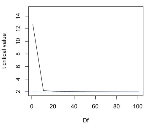
Figure 1. Critical values at Type I rate of 5% of t-distribution  . Blue dashed line is z = 1.96.
Here’s the equation for calculating the confidence interval based on the t-distribution. These set the limits around our estimate of the sample mean. Together, they’re called the 95% confidence interval,  .

Here’s a simplified version of the same thing, but generalized to any Type I level…
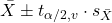
This statistic allows us to say that we are 95% confident that the interval includes the true value for . For this confidence interval you need to identify the critical t value at 5%. Thus, you need to know the degrees of freedom for this problem, which is simply  , the sample size minus one.
It is straightforward to calculate these by hand, but…
Set the Type I error rate, calculate the degrees of freedom (df):
 samples for one sample test
- pairs of samples for paired test
 samples for two independent sample test
and lookup the critical value from the t table (or from the t distribution in R). Of course, it is easier to use R.
In R, for the one tail critical value with seven degrees of freedom, type at the R prompt
qt(c(0.05), df=7, lower.tail=FALSE)
[1] 1.894579
For the two-tail critical value
qt(c(0.025), df=7, lower.tail=FALSE)
[1] 2.364624
Or, if you prefer to use R Commander, then follow the menu prompts to bring up the t quantiles function (Fig 2 and Fig 3).
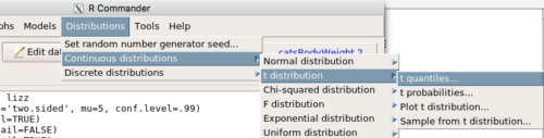
Figure 2. Drop down menu to get t-distribution.
Note 2: Quantiles divide probability distribution into equal parts or intervals. Quartiles have four groups, deciles have ten groups, and percentiles have 100 groups.
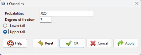
Figure 3. Menu for t quantiles, with values entered for the two-tail example.
You should confirm that what R calculates agrees with the critical values tabulated in the Table of Critical values for the t distribution provided in the Appendix.
A worked example
Let’s revisit our lizard example from last time (see Chapter 8.5). Prior to conducting any inference test, we decide acceptable Type I error rates (cf justify alpha discussion in Ch8.1); For this example, we set Type I error rate to be 1% for a 99% confidence interval.
The Rcmdr output was
t.test(lizz$bm, alternative='two.sided', mu=5, conf.level=.99)
data: lizz$bm
t = -1.5079, df = 7, p-value = 0.1753
alternative hypothesis: true mean is not equal to 5
99 percent confidence interval:
1.984737 6.199263
sample estimates:
mean of x
4.092
Sort through the output and identify what you need to know.
Question 1: What was the sample mean?
- 5
- -1.5079
- 7
- 0.1753
- 1.984737
- 6.199263
- 4.092
Question 2: What was the most likely population mean?
- 5
- Answer
- -1.5079
- 7
- 0.1753
- 1.984737
- 6.199263
- 4.092
Question 3: This was a “one-tailed” test of the null hypothesis?
- True
- False
The output states “alternative hypothesis: true mean is not equal to 5” — so it was a two-tailed test.
Question 4: What was the lower limit of the confidence interval?
- 5
- -1.5079
- 7
- 0.1753
- 1.984737
- 6.199263
- 4.092
The 99% confidence interval,  , is
 , which means we are 99% certain that the population mean is between
 (lower limit) and
 (upper limit). In Chapter 8.5 we calculated the , is
 .
Confidence intervals by nonparametric bootstrap sampling.
Bootstrapping is a general approach to estimation or statistical inference that utilizes random sampling with replacement (Kulesa et al. 2015). In classic frequentist approach, a sample is drawn at random from the population and assumptions about the population distribution are made in order to conduct statistical inference. By resampling with replacement from the sample many times, the bootstrap samples can be viewed as if we drew from the population many times without invoking a theoretical distribution. A clear advantage of the bootstrap is that it allows estimation of confidence intervals without assuming a particular theoretical distribution and thus avoids the burden of repeating the experiment. Which method to prefer? For cases where assumption of a particular distribution is unwarranted (eg, what is the appropriate distribution when we compare medians among samples?), bootstrap may be preferred (and for small data sets, percentile bootstrap may be better). We cover bootstrap sampling of confidence intervals in Chapter 19.2 Bootstrap sampling.
Conclusions
The take home message is simple.
- All estimates should — must? — be accompanied by a Confidence Interval
- The more confident we wish to be, the wider the confidence interval will be
Note that the confidence interval concept combines DESCRIPTION (the population mean is between these limits) and INFERENCE (and we are 95% certain about the values of these limits). It is good statistical practice to include estimates of confidence intervals for any estimate you share with readers. Any statistic that can be estimated should be accompanied by a confidence interval and, as you can imagine, formulas are available to do just this. For example, earlier this semester we calculated NNT.
Questions
- To gain practice with calculations of confidence intervals, calculate the approximate confidence interval, the 95% and the 99% confidence intervals based on the t distribution, for each of the following.
-
- = 13,
 = 1.3,
 = 10
- = 13, = 1.3, = 30
- = 13, = 2.6, = 10
- = 13, = 2.6, = 30
Quiz Chapter 8.6
Confidence limits for the estimate of population mean
Chapter 8 contents
- Introduction
- The null and alternative hypotheses
- The controversy over proper hypothesis testing
- Sampling distribution and hypothesis testing
- Tails of a test
- One sample t-test
- Confidence limits for the estimate of population mean
- References and suggested readings
7.2 – Epidemiology basics
Introduction
A principle aim of epidemiology is to identify frequency and causes of illnesses. Kinds of evidence gathered range from case studies to randomized controlled trials, to meta-analysis and systematic reviews. In turn, how these kinds of evidence are evaluated and turned into policy recommendations generally accounts for additional concerns eg, GRADE – Grading of Recommendations Development, Assessment and Evaluation Schünemann et al 2023). Learning about conditional probability in biostatistics is essential for discussing evidence because it provides a rigorous framework for updating strength of evidence based on new, specific information. It allows for the objective assessment of how new evidence — results from a clinical test — influences the likelihood of a hypothesis — presence/absence of disease for a patient. Conditional probability analysis allows interpretation of a positive test result in the context of disease prevalence, which may lead to the paradoxical conclusion that a test with high sensitivity applied to a person belonging to a low at risk group is more likely a false positive than evidence of a true positive.
Thus, to introduce conditional probability, I have elected to push you into epidemiology and risk analysis. We introduced epidemiology definitions and here, we build on basic terminology of epidemiology. Epidemiology is the study of the causes and distribution of health-related events in a population. It is has been called the basic science of public health (p. 16, Decker 2008).
Prevalence rate
Prevalence of a disease (condition), is defined as the proportion of the population that has the disease (condition) at a point or duration in time. The prevalence statistic is the ratio of the number of existing cases divided by the total population.
For example, prevalence of Type 2 diabetes in Hawai`i. The 2020 populations was about 1.4 million. A survey was conducted on a random of 1000 individuals and 80 were reported to have Type 2 diabetes. What is the estimated prevalence of Type 2 diabetes in Hawai`i?
Start from perspective — what if we actually have something close to a census count? For the actual estimates, see the report at the Hawaii State DOH website. With every estimate of a statistic, we need a confidence interval (CI). An approximate (good for large samples) formula for the 95% CI of prevalence is

where  is the 2010 prevalence in the population (8.3%), N is the population size (1,360,301), and z is the standard normal probability. For a 95% CI, then we want z95%.
If you recall, we can get this from our standard normal probability table, or directly from R. We want to know z that is in the ± 2.5% tails of the distribution (that’s 0.05 ÷ 2, see Ch 8.4 – Tails of a test). Our R code then is
qnorm(c(0.025), mean=0, sd=1, lower.tail=FALSE)
which returns
[1] 1.959964
You should confirm that setting lower-tail = TRUE yields -1.96 (rounded).
Alternately, if using Rcmdr: Distributions → Continuous distributions → Normal distribution → Normal quantiles… (Fig 1).
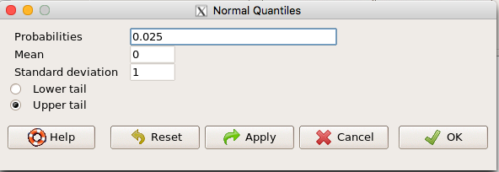
Figure 1. R Commander popup menu for Normal quantiles.
Thus, for our example, the 95% CI was ( ; our confidence in our estimate of the prevalence of diabetes in Hawaii is between 8.25% and 8.35%. Again, note that for our purposes it is OK to calculate the approximate confidence interval, replace with
 (for large N, the differences are observed in the 0.001 decimal).
Prevalence: R code
Rather than census counts, more likely we have results of smaller surveys. We use the epi.conf() function from the epiR package. Code adapted from example provided in epiR_descriptive vignette.
Note 1: Many R packages include vignettes, which, together with the package manual, is often helpful to understand what a function is intended to do and how to get the most from the function. R code to call all vignettes available for a package, eg, epiR:
vignette(package="epiR")
which will return names of available vignettes. For epiR, these are
epiR_descriptive Descriptive epidemiology (source, html)
epiR_surveillance Disease surveillance (source, html)
epiR_measures_of_association Measures of association (source, html)
epiR_sample_size Sample size calculations (source, html)
To call up the vignette we need for this example,
vignette("epiR_descriptive", package="epiR")
which brings up the page (assuming you installed the html help files during installation of base R).
library(epiR)
pop.Hawaii = 1.4e06
pop.Survey = 1000
type2.Survey = 80
Table.2 <- as.matrix(cbind(type2.Survey, pop.Survey))
epi.conf(Table.2, ctype = "prevalence", method = "exact", N = pop.Hawaii, design = 1, conf.level = 0.95) * 100
R output
   est    lower    upper
1    8 6.394198 9.857978
Thus, estimated Type 2 diabetes prevalence from the survey was 8, with 95% confidence interval 6.4 to 9.9 cases per 100 individuals. From 2020 U.S. Census, Hawai`i population was 1,455,271.
Note 2: Type 2 diabetes is one of many conditions for which prevalence is greater among Native Hawaiian and Pacific Islander populations compared to other groups in Hawai’i (Galinski et al 2016); these are called health disparitiess.
Incidence rate
Incidence of a disease (or condition) is defined as the occurrence of new cases of a disease. The simplest way to view incidence is that if everyone was followed for the same period of time, then incidence rate is the number of new cases since the start of the study divided by the total population. This is too simplistic, so we define a better metric called person-time. Incidence rate (IR) is then the ratio of the number of new cases divided by total person-time.
Again, incidence rate is an estimate. Therefore, we need a confidence interval. Assuming the population is large, then confidence interval can be calculated as

where IR is the incidence rate, T is the person-time, N is the number of events or cases, and z again is the standard normal probability (z ± 1.96 for 95% confidence interval).
For our example, N = 3 cases, T = 236 p-d, so 95% CI is (11.3%, 14.1%).
Person-time
Person-time can be days, months, years. Person-time is best defined with an example.
Five men join a study that will last 70 days. These men were selected because they had suffered a myocardial infarction (MI) and at the start of the study, they receive the same treatment. The outcome of the study is whether or not the subjects suffer a second MI.
The results are shown below
Subject A, 53 days
Subject B, 70 days
Subject C, 24 days
Subject D, 70 days
Subject E, 19 days
Add up the person days,

Now calculate the incidence rate,

that’s 3 cases (A, C, E) divided by 236 p-d = 0.0127. Multiply this by 1000 and we get our final answer for the incidence rate, 12.7 per person-days.
Incidence rate: R code
Incidence rate of myocardial infarction (MI) study. Code adapted from example provided in epiR_descriptive vignette.
ncas = 3
ntar = 236
tmp <- as.matrix(cbind(ncas, ntar))
epi.conf(tmp, ctype = "inc.rate", method = "exact", N = 1000, design = 1, conf.level = 0.95) * 1000
R output
          est    lower    upper
ncas 12.71186 2.621492 37.14946
The incidence rate of myocardial infarction was 12.7 (95% CI 2.6 to 37.2) cases per 1000 person-days.
Age-specific rates
Incidence or prevalence rates may be reported for specific age groups. For example, we can distinguish between number of live births in Hawaii in 2017, and numbers of live births by age group of the mother.
Age-adjusted rates
If populations with different age demographics, then the convention is to adjust the populations to a standard reference population with known age and other demographic properties. For example, the CDC uses the 2000 census as the standard population (CDC definitions, age adjustment, retrieved January 2023).
Questions
- Calculate the confidence interval of type 2 prevalence in Hawai`i with the 2020 census population value. How much did it change?
- Recalculate the confidence interval for a 99% confidence interval. Which estimate communicates greater confidence in the estimate?
Quiz
Quiz Chapter 7.2
Epidemiology basics