17 – Linear Regression
Introduction
Regression is a toolkit for developing models of cause and effect between one ratio scale data type dependent response variables, and one (simple linear regression) or more or more (multiple linear regression) ratio scale data type independent predictor variables. By convention the dependent variable(s) is denoted by Y, the independent variable(s) represented by X1, X2,  Xn for n independent variables. Like ANOVA, linear regression is simply a special case of the general linear model, first introduced in Chapter 12.7.
Components of a statistical model
Regression statistical methods return model estimates of the intercept and slope coefficients, plus statistics of regression fit (eg, R2, aka “R-squared,” the coefficient of determination).
Chapter 17.1 – 17.9 cover the simple linear model

Chapter 18.1 – 18.5 cover the multiple regression linear model

where α or β0 represent the Y-intercept and β or β1, β2, … βn represent the regression slopes.
Regression and correlation test linear hypotheses
We state that the relationship between two variables is linear (the alternative hypothesis) or it is not (the null hypothesis). The difference? Correlation is a test of linear association (are variables correlated, we ask?), imply possible causation, but are not sufficient evidence for causation: we do not imply that one variable causes another to vary, even if the correlation between the two variables is large and positive, for example. Correlations are used in statistics on data sets not collected from explicit experimental designs incorporated to test specific hypotheses of cause and effect.
Linear regression, however, is to cause and effect as correlation is to association. With regression and ANOVA, we are indeed making a case for a particular understanding of the cause of variation in a response variable: modeling cause and effect is the goal. Regression, ANOVA, and other general linear models are designed to permit the statistician to control for the effects of confounding variables provided the causal variables themselves are uncorrelated.
When to use correlation and when to apply linear regression to data set? For two ratio scale variables, one can always apply either approach. Correlation is always appropriate if both variables are measured in the course of the study whereas a regression modeling approach would be implied where one variable was the result of manipulation by the researcher.
Assumptions of linear regression
The key assumption in linear regression is that a straight line indeed is the best fit of the relationship between dependent and independent variables. The additional assumptions of parametric tests (Chapter 13) also hold. In Chapter 18 we conclude with an extension of regression from one to many predictor variables and the special and important topic of correlated predictor variables or multicollinearity.
Build a statistical model, make predictions
In our exploration of linear regression we begin with simple linear regression, also called ordinary least squares regression, starting with one predictor variable. Practical aspects of model diagnostics are presented. Regression may be used to describe or to provide a predictive statistical framework. In Chapter 18 we conclude with an extension of regression from one to many predictor variables. We conclude with a discussion of model selection. Throughout, use of Rcmdr and R have multiple ways to analyze linear regression models are presented; we will continue to emphasize the general linear model approach, but note that use of linear model in Rcmdr provides a number of default features that are conveniently available.
Questions
1. Write up three learning outcomes for this page. Hint: Point your favorite generative AI to this page and ask for help.
Suggested homework
Homework 11: Simple linear regression.
Quiz
In addition to the quiz on this page, a total of 81 questions among the several subchapters, a mix of true or false and multiple choice question format.
Quiz Chapter 17
Linear Regression
References
Linear regression is a huge topic; references I include are among my favorite on the subject, but are only a small and incomplete sampling. For simplicity, I merged references for Chapter 17 and Chapter 18 into one page at References and suggested readings (Ch17 & 18)
Chapter 17 contains
- Introduction
- Simple Linear Regression
- Relationship between the slope and the correlation
- Estimation of linear regression coefficients
- OLS, RMA, and smoothing functions
- Testing regression coefficients
- ANCOVA – analysis of covariance
- Regression model fit
- Assumptions and model diagnostics for Simple Linear Regression
- References and suggested readings (Ch17 & 18)
13.4 – Tests for Equal Variances
Introduction
In order to carry out statistical tests correctly, we must test our data first to see if our sample conforms to the assumptions of the statistical test. If our data do not meet these assumptions, then inferences drawn may be incorrect. How far off our inferences may be depends on a number of factors, but mostly it depends on how far from the expectations our data are.
One assumption we make with parametric tests involving ratio scale data is that the data could be from a normally distributed population. The other key assumption introduced, but not described in detail for the two-sample t-test, was that the variability in the two groups must be the same, ie, homoscedasticity. Thus, in order to carry out the independent sample t-test, we must assume that the variances are equal.
There are two general reasons we may want to concern ourselves with a test for the differences between two variances
- The t-test (and other tests like one-way ANOVA) requires that the two samples compared have the same variances. If the Variances are Not Equal we need to perform a modified t-test (see Welch’s formula).
- We may also be interested in the differences between the variances in two populations.
Example 1: In genetics we might be interested in the difference between the variability of response of inbred lines (little genetic variation but environmental variation) versus an outbred populations (lots of genetic and environmental variation).
Example 2: Environmental stress can cause organisms to have developmental instability. This might cause organisms to be more variable in morphology or the two sides (right & left) of an organism may develop non-symmetrically. Therefore, polluted environments might cause organisms to have greater variability compared to non-polluted environments.
The first way to test the variances is to use the F test. This works for two groups.

For more than two groups, we’ll use different tests (eg, Bartlett’s test, Levene’s test).
Remember that the formula for the sample variance is
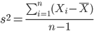
The Null Hypothesis is that the two samples have the same variances:

The Alternative Hypothesis is that the two samples do not have the same variances:

Note: I prefer to evaluate this as a one-tailed test: identify the larger of the two variances and take that as the numerator Then, the null hypothesis is that

and therefore, the alternative hypothesis is that (ie, a one-tailed test).

Another way to state equal variance test is that we are testing for homogeneity of variances. You may run across the term homoscedasticity; it is the same thing, just a different three dollar word for “equal variances.”
Stated yet another way, if we reject the null hypothesis, then the variances are unequal or show heterogeneity. An additional and equivalent $3 word for inequality of variances is called heteroscedasticity.
More about the F-test
For the F-test, the null hypothesis is that the variances are equal. This means that the “expected” F value will be one: F = 1.0. (The F-distribution differs from t-distribution because it requires 2 values for DF, and ranges from 1 to infinity for every possible combination of v1 and v2).
To evaluate the null hypothesis we need the degrees of freedom. For the F test we need two different degrees of freedom, one set for each group): from Table 2, Appendix – F distribution, look up 5% Type I error line in this table because we make it one tailed.
I need the F-test statistic at 
Examples of difference between two variances, Table 1.
Sample 1: Aggressiveness of Inbred Mice (number of bites in 30 minutes)
Sample 2: Aggressiveness of Outbred Mice (number of bites in 30 minutes)
Table 1. Aggression by inbred and outbred mice.
| Sample 1
Aggressiveness of Inbred Mice |
Sample 2
Aggressiveness of Outbred Mice |
| 3 | 4 |
| 5 | 10 |
| 4 | 4 |
| 3 | 7 |
| 4 | 7 |
| 5 | 10 |
| 4 = mean | 7 = mean |
- Identify the null and alternative hypotheses
- Calculate Variances
- Calculate F-test
- The “test statistic” for this hypothesis test was F = 7.2 / 0.8 = 9.0
- Determine Critical Value of the F table (Table 2, Appendix – F distribution)
Example of how to find the critical values of the F distribution for  and numerator
 and denominator
 .
Table 2. Portion of F distribution, see Appendix – F distribution.
| α = 0.05 | v1 | ||||||||
| 1 | 2 | 3 | 4 | 5 | 6 | 7 | 8 | ||
| v2 | 1 | 230 | |||||||
| 2 | 19.3 | ||||||||
| 3 | 9.01 | ||||||||
| 4 | 6.26 | ||||||||
| 5 | 6.61 | 5.79 | 5.41 | 5.19 | 5.05 | 4.95 | 4.88 | 4.82 | |
| 6 | |||||||||
Or, instead of using tables, use R
Rcmdr: Distributions → F distribution → F probabilities
and enter the numbers as shown below (Fig 1).
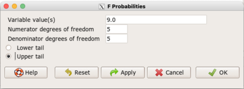
Figure 1. Screenshot R Commander F distribution probabilities.
This will return the p-value, and you would interpret this against your Type I error rate of 5% as you do for other tests.
From Table 2, Appendix – F distribution we find 
And the p-value = 0.015
pf(c(9), df1=5, df2=5, lower.tail=FALSE)
[1] 0.01537472
Question: Reject or Accept null hypothesis?
Question: What is the biological interpretation or conclusion from this result?
R code
Rather than play around with the tables of critical values, which are awkward and old-school (and I am showing you these stats tables so that you get a feel for the process, not so you’d actually use them in real practice), use Rcmdr to generate the F test and therefore return the F distribution probability value. As you may expect, R provides a number of options for testing the equal variances assumption, including the F test. The F test is limited to only two groups and, because it is a parametric test, it also makes the assumption of normality, so the F test should not be viewed as necessarily the best test for the equal variances assumption among groups. We present it here because it is a logical test to understand and because of its relevance to the Mean Square ratios in the ANOVA procedures.
So, without further justification, here is the presentation on how to get the F test in Rcmdr. At the end of this section I present a better procedure than the F test for evaluating the equal variance assumption called the Levene test.
Return to the bite data in the table above and enter the data into an R data frame. Note that the data in the table above are unstacked; R expects the data to be stacked, so either create a stacked worksheet and transcribe the data appropriately into the cells of the worksheet, or, go ahead and enter the values into two separate columns then use the Stack variables in active data set… command from the Data menu in Rcmdr.
Then, proceed to perform the F test.
Rcmdr: Statistics → Variances → Two variances F-test…
The first context menu popup is where you enter the variables (Fig 2).
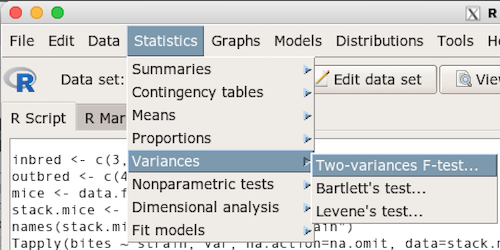
Figure 2. Screenshot data options R Commander F test
Because there are only two variables in the data set and because Strain contains the text labels of inbred or outbred whereas the other variable is numeric data type, R will correctly select the variables for you by default. Select the “Options” tab to set the parameters of the F test (Fig 3).
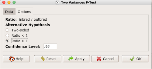
Figure 3. Screenshot menu options R Commander F test.
When you are finished setting the alternative hypothesis and confidence levels, proceed with the F test by clicking the OK button.
    F test to compare two variances

data:  mice.aggression
F = 0.1111, num df = 5, denom df = 5, p-value = 0.03075
alternative hypothesis: true ratio of variances is not equal to 1
95 percent confidence interval:
 0.01554788 0.79404243
sample estimates:
ratio of variances
         0.1111111
End of R output.
Levene’s test of equal variances
We will discuss this test in more detail following our presentation on ANOVA. For now, we note that the test works on two or more groups and is a conservative test of the equal variance assumption. Nonparametric tests in general make fewer assumptions about the data and in particular make no assumption of normality like the F test. It is in this context that the Levene’s test would be preferable over the F test. Below we present only how to calculate the statistic in R and Rcmdr and provide the output for the same mouse data set.
Assuming the data are stacked, obtain the Levene’s test in Rcmdr by clicking on (Fig 4).
Rcmdr: Statistics → Variances → Levene’s test…
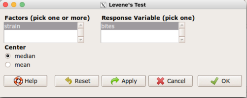
Figure 4. Screenshot menu options R Commander Levene’s test.
Select the median and the factor variable (in our case “Strain”) and the numeric outcome variable (“Bites”), then click OK button.
Tapply(bites ~ strain, var, na.action=na.omit, data=mice.aggression) # variances by group
inbred outbred
   0.8     7.2

leveneTest(bites ~ strain, data=mice.aggression, center="median")
Levene's Test for Homogeneity of Variance (center = median)
      Df F value  Pr(>F)
group  1       4 0.07339 .
      10
---
Signif. codes:  0 '***' 0.001 '**' 0.01 '*' 0.05 '.' 0.1 ' ' 1
End of R output
Compare the p-values. In both cases — F test and Levene’s test — we’re testing the same hypothesis (equal variances), but the p-values do not agree between the parametric F test and the nonparametric Levene’s test! If we were to go by the results of the F test, p-value was 0.031, less than out Type I error of 5% and we would tentatively conclude that the assumption of equal variances may not apply. On the other hand, if we go with the Levene’s test the p-value was 0.074, which is greater than our Type I error rate of 5% and we would therefore conclude the opposite, that the assumption of equal variances might apply! Both conclusions can’t hold, so which test result of equal variances do we prefer, the parametric F test or the nonparametric Levene’s test? Answer — we’d go with Levene’s because the F test is parametric and, therefore, also assumes normality.
Cahoy’s bootstrap method
Draft. Cahoy (2010). Variance-based statistic bootstrap test of heterogeneity of variances. we discuss bootstrap methods in Chapter 19.2; in brief, bootstrapping involves resampling the dataset and computing a statistic on each sample. This method may be more powerful, that is, more likely to correctly reject the null hypothesis when warranted, compared to Levene’s test.
for now, install package testequavar.
Function for testing two samples.
equa2vartest(inbred, outbred, 0.05, 999)
R output
[[1]]
[1] "Decision: Reject the Null"
$Alpha
[1] 0.05
$NumberOfBootSamples
[1] 999
$BootPvalue
[1] 0.006
The output “Decision: Reject the Null” reflects output from a box-type acceptance region.
Compare results from Levene’s test: p-value 0.07339 suggests accept hypothesis of equal variances, whereas bootstrap method indicates variances heterogenous, ie, reject equal variance hypothesis. However, re-running the test without setting the seed for R’s pseudorandom number generator will result in different p-values. For example, I re-ran Cahoy’s test five times with the following results:
0.008
0.006
0.002
0.01
0.004
Questions
- Test assumption of equal variances by Bartlett’s method and by Levene’s test on
OliveMomentvariable from the Comet tea data set introduced in Chapter 12.1. Do the methods agree? If not, which test result would you choose?- BONUS. Retest homogeneous variance hypothesis by
equa3vartest(Copper.Hazel, Copper, Hazel, 0.05, 999). Reject or fail to reject the null hypothesis by bootstrap method?
- BONUS. Retest homogeneous variance hypothesis by
- Test assumption of equal variances by Bartlett’s method and by Levene’s test on
Heightfrom the O’hia data set introduced in Chapter 12.7. Do the methods agree? If not, which result would you choose?- BONUS. Retest homogeneous variance hypothesis by
equa3vartest(M.1, M.2, M.3, 0.05, 999). Reject or fail to reject the null hypothesis by bootstrap method?
- BONUS. Retest homogeneous variance hypothesis by
Quiz Chapter 13.4
Tests for Equal Variances
R code reminders
The bootstrap method expects the variables in unstacked format. A simple method to extract the variables from the stacked data is to use a command like the following. For example, extract OliveMoment values for Copper-Hazel treatment.
Copper.Hazel <- cometTea$OliveMoment[1:10]
For Copper, Hazel, replace above with [11:20], and [21-30] respectively. Note: changed variable name from Copper-Hazel to Copper.Hazel. The hyphen is a reserved character in R.
Chapter 13 contents
12.2 – One way ANOVA
Introduction
In ANalysis Of VAriance, or ANOVA for short, we likewise have tools to test the null hypothesis of no difference between between categorical independent variables — often called factors when there’s just a few levels to keep track of — and a single, dependent response variable. But now, the response variable is quantitative, not qualitative like the  tests.
Analysis of variance, ANOVA, is such an important statistical test in biology that we will take the time to “build it” from scratch. We begin by reminding you of where you’ve been with the material.
We already saw an example of this null hypothesis. When there’s only one factor (but with two or more levels), we call the analysis of means and “one-way ANOVA.” In the independent sample t-test, we tested whether two groups had the same mean. We made the connection between the confidence interval of the difference between the sample means and whether or not it includes zero (ie, no difference between the means). In ANOVA, we extend this idea to a test of whether two or more groups have the same mean. In fact, if you perform an ANOVA on only two groups, you will get the exact same answer as the independent two-sample t-test, although they use different distributions of critical values (t for the t-test, F for the ANOVA — a nice little fact for you square the t-test statistic, you’ll get the F-test statistic:  ).
Let’s say we have an experiment where we’ve looked at the effect of different three different calorie levels on weight change in middle-aged men.
I’ve created a simulated dataset which we will use in our ANOVA discussions. The data set is available at the end of this page (scroll down or click here).
We might graph the mean weight changes ( SEM); Below are two possible outcomes of our experiment (Fig 1).
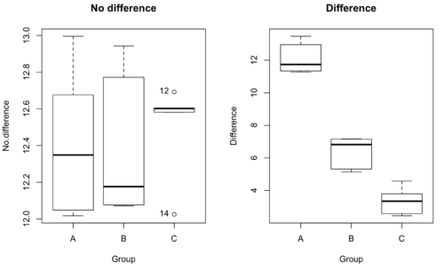
Figure 1. Hypothetical results of an experiment, box plots. Left, no difference among groups; Right, large differences among groups.
As statisticians and scientists, we would first calculate an overall or grand mean for the entire sample of observations; we know this as the sample mean whose symbol is  . But this overall mean is made up of the average of the sample means. If the null hypothesis is true, then the all of the sample means all estimate the overall mean. Put another way, being a member of a treatment group doesn’t matter, ie, there is no systematic effect, all differences among subjects are due to random chance.

The hypotheses among are three groups or treatment levels then are:

Null that there are no differences among the group means. And the alternative hypotheses include any (or all) of the following possibilities

or maybe

or… have we covered all possible alternate outcomes among three groups?
In either case, we could use one-way ANOVA to test for “statistically significant differences.”
Three important terms you’ll need for one-way ANOVA
FACTOR: We have one factor of interest. For example, a factor of interest might be
- Diet fed to hypertensive subjects (men and women)
- Distribution of coral reef sea cucumber species in archipelagos
- Antibiotic drug therapy for adolescents with Acne vulgaris (click see Webster 2002 for review).
Note 1: Character vs factor. In R programming, while it is true that a treatment variable can be a character vector like Gender*, such vectors are handled by R as string. In contrast, by claiming Gender as a factor, R handles the variable as a nominal data type. Hence, ANOVA and other GLM functions expect any treatment variable to be declared as a factor:
Gender <- c("Gender non-conforming", "Men", "Non-binary", "Transgender", "Women", "Declined"); Gender
[1] "Gender non-conforming" "Men" "Non-binary" "Transgender"
[5] "Women" "Declined"
# it’s a string vector, not a factor
is.factor(Gender)
[1] FALSE
Change string vector to a factor.
Gender <- as.factor(Gender); is.factor(Gender) [1] TRUE
* For discussions of ethics of language inclusivity and whether or not such information should be gathered, see Henrickson et al 2020.
LEVELS: We can have multiple levels (2 or more) within the single factor. Some examples of levels for the Factors listed:
- Three diets (DASH), diet rich in fruits & vegetables, control diet)
- Five archipelagos (Hawaiian Islands, Line Islands, Marshal Islands, Bonin Islands, and Ryukyu Islands)
- Five antibiotics (ciprofloxacin, cotrimoxazole, erythromycin, doxycycline, minocycline).
RESPONSE: There is one outcome or measurement variable. This variable must be quantitative (ie, on the ratio or interval scale). Continuing our examples then
- Reduction in systolic pressure
- Numbers of individual sea cucumbers in a plot
- number of microcomedo.
Note 2: A comedo is a clogged pore in the skin; a microcomedo refers to the small plug. Yes, I had to look that up, too.
The response variable can be just about anything we can measure, but because ANOVA is a parametric test, the response variable must be normally distributed!
Note on experimental design
As we discuss ANOVA, keep in mind we are talking about analyzing results from an experiment. Understanding statistics, and in particular ANOVA, informs how to plan an experiment. The basic experimental design is called a completely randomized experimental design, or CDR, where treatments are assigned to experimental units at random.
In this experimental design, subjects (experimental units) must be randomly assigned to each of these levels of the factor. That is, each individual should have had the same probability of being found in any one of the levels of the factor. The design is complete because randomization is conducted for all levels, all factors.
Thinking about how you would describe an experiment with three levels of some treatment, we would have
Table 1. Summary statistics of three levels for some ratio scale response variable.
| Level 1 |
sample mean1 |
sample standard deviation1 |
| Level 2 |
sample mean2 |
sample standard deviation2 |
| Level 3 |
sample mean3 |
sample standard deviation3 |


Note 3: Table 1 is the basis for creating the box plots in Figure 1.
ANOVA sources of variation
ANOVA works by partitioning total variability about the means (the grand mean, the group means). We will discuss the multiple samples and how the ANOVA works in terms of the sources of variation. There are two “sources” of variation that can occur:
- Within Group Variation
- Among Groups Variation
So let’s look first at the variability within groups, also called the Within Group Variation.
Consider and experiment to see if DASH diet reduces systolic blood pressure in USA middle-aged men and women with hypertension (Moore et al 2001). After eight weeks we have
We get the corrected sum of squares, SS, for within group

and the degrees of freedom, DF, for within groups

where i is the identity of the groups,  is the individual observations within group i,
 is the group i mean, ni is the sample size within each group, N is the total sample size of all subjects for all groups, and k is the number of groups.
Importantly, this value is also referred to as “error sums of squares” in ANOVA. It’s importance is as follows — In our example, the within group variability would be zero if and only if all subjects within the same diet lost exactly the same amount of weight. This is hardly ever the case of course in a real experiment. Because there are almost always some other unknown factors or measurement error that affect the response variable, there will be some unknown variation among individuals who received the same treatment (within the same group). Thus, the error variance will generally be larger than zero.
The first point to consider: your ANOVA will never result in statistical differences among the groups if the error variance is greater than the second type of variability, the variability between groups.
The second type of variability in ANOVA is that due to the groups or treatments. Individuals given a calorie-restricted diet will lose some weight; individuals allowed to eat a calorie-rich diet likely will gain weight, therefore there will be variability (a difference) due to the treatment. So we can calculate the variability among groups. We get the corrected sum of squares for among groups

and the degrees of freedom for among groups

where i is the identity of the groups, is the grand mean as defined in Measures of Central Tendency (Chapter 3.1), is the group i mean, ni is the sample size within each group, N is the total sample size of all subjects for all groups, and k is the number of groups.
The sums of squares here is simply subtracting the mean of each population from the overall mean.
- If the Factor is not important in explaining the variation among individuals then all the population means will be similar and the sums of squares among populations would be small.
- If the Factor is important in explaining some of the variation among the individuals then all the population means will NOT be the same and the sums of squares among populations would be large.
Finally, we can identify the total variation in the entire experiment. We have the total sum of squares.

Thus, the insight of ANOVA is that variation in the dataset may be attributed to a portion explained by differences among the groups and differences among individual observations within each group. The inference comes from recognizing that if the among group effect is greater than the within group effect, then there will be a difference due to the treatment levels.
Mean squares
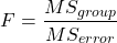
To decide whether the variation associated with the among group differences are greater than the within group variation, we calculate ratios of the sums of squares. These are called Mean Squares or MS for short. The ratio of the Mean Squares is called F, the test statistic for ANOVA.
For the one-way ANOVA we will have two Mean Squares and one F, tested with degrees of freedom for both the numerator  , and denominator
 ).
The Mean Square for (among) groups is

The Mean Square for error is

And finally, the value for F, the test statistic for ANOVA, is
Worked example with R
A factor with three levels, A, B, and C
group <- c("A", "A", "A", "B", "B", "B", "C", "C", "C")
and their responses, simulated
response <- c(10.8, 11.8, 12.8, 6.5, 7, 8, 3.8, 2.8, 3)
We create a data frame
all <- data.frame(group, response)
Of course, you could place the data into a worksheet and then import the worksheet into R. Regardless, we now have our dataset.
Now, call the ANOVA function, aov, and assign the results to an object (eg, Model.1)
Model.1 <- aov(response ~ group, data=all)
Now, visualize the ANOVA table
summary(Model.1)
and the output from R, the ANOVA table, is shown below
Note 4: Rcmdr: Statistics → Means → One-way ANOVA… see figures 2 and 3 below
Table 2. Output from aov() command, the ANOVA table, for the “Difference” outcome variable.
           Df   Sum Sq    Mean Sq   F value       Pr(>F)
group       2   111.16      55.58     89.49    0.0000341 ***
Residuals   6     3.73       0.62
---
Signif. codes: 0 '***' 0.001 '**' 0.01 '*' 0.05 '.' 0.1 ' ' 1
Let’s take the ANOVA table one row at a time
- The first row has subject headers defining the columns.
- The second row of the table “groups” contains statistics due to group, and provides the comparisons among groups.
- The third row, “Residuals” is the error, or the differences within groups.
Moving across the columns, then, for each row, we have in turn,
- the degrees of freedom (there were 3 groups, therefore 2 DF for group),
- the Sums of Squares, the Mean Squares,
- the value of F, and finally,
- the P-value.
R provides a helpful guide on the last line of the ANOVA summary table, the “Signif[icance] codes,” which highlights the magnitude of the P-value.
Note 5: On the use of “error” and “residuals.” Error refers to the difference between an observed value and the true population value. Residual is the difference between an observed value and a value predicted by a model. In ANOVA, the “error variance” or “residual variance” is the variation within groups unexplained by the tested factor. It is what remains after the effects of the model are accounted for.
What to report? ANOVA problems can be much more complicated than the simple one-way ANOVA introduced here. For complex ANOVA problems, report the ANOVA table itself! But for the one-way ANOVA it would be sufficient to report the test statistic, the degrees of freedom, and the p-value, as we have in previous chapters (eg, t-test, chi-square, etc.). Thus, we would report:
F = 89.49, df = 2 and 6, p = 0.0000341
where F = 89.49 is the test statistic, df = 2 (degrees of freedom for the among group mean square) and 6 (degrees of freedom for the within group mean square), and p = 0.0000341 is the p-value.
In Rcmdr, the appropriate command for the one-way ANOVA is simply
Rcmdr: Statistics → Means
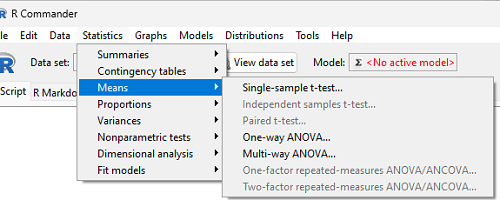
Figure 2. Screenshot Rcmdr select one-way ANOVA.
which brings up a simple dialog. R Commander anticipates factor (Groups) and Response variable. Optional, choose Pairwise comparisons of means for post-hoc test (Tukey’s) and, if you do not want to assume equal variances (see Chapter 13), select Welch F-test.
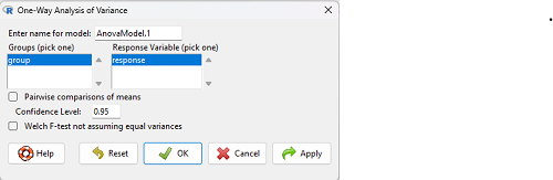
Figure 3. Screenshot Rcmdr select one-way ANOVA options.
Questions
1. Review the example ANOVA Table and confirm the following
- How many levels of the treatment were there?
- How many sampling units were there?
- Confirm the calculation of
 and using the formulas contained in the text.
- Confirm the calculation of F using the formula contained in the text.
- The degrees of freedom for the F statistic in this example were 2 and 6 (F2,6). Assuming a two-tailed test with Type I error rate of 5%, What is the critical value of the F distribution (see Appendix 20.4)
2. Repeat the one-way ANOVA using the simulated data, but this time, calculate the ANOVA problem for the “No.difference” response variable.
3. Leaf lengths from three strains of Arabidopsis thaliana plants grown in common garden are shown in Fig 2. Data are provided for you in the following R script.
arabid <- c("wt","wt","wt","AS1","AS1","AS1","AS2","AS2","AS2")
leaf <- c(4.909,5.736,5.108,6.956,5.809,6.888,4.768,4.209,4.065)
leaves <- data.frame(arabid,leaf)
- Write out a null and alternative hypotheses
- Conduct a test of the null hypothesis by one-way ANOVA
- Report the value of the test statistic, the degrees of freedom, and the P-value
- Do you accept or reject the null hypothesis? Explain your choice.
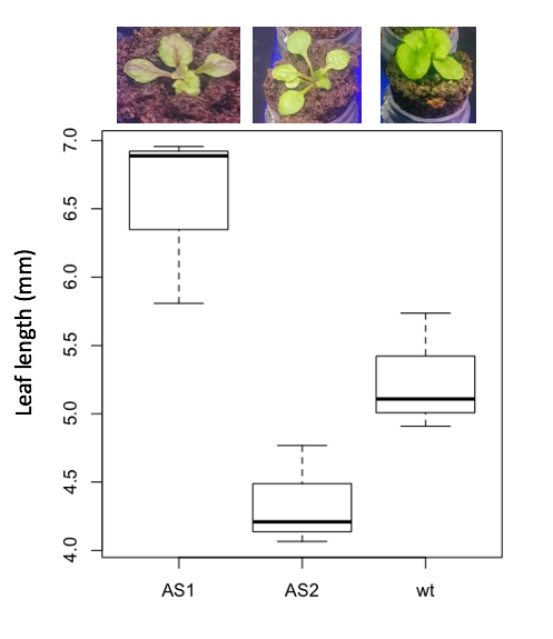
Figure 4. Box plot of lengths of leaves of a 10-day old plant from on of three strains of Arabidopsis thaliana.
4. Return to your answer to question 7 from Chapter 12.1 and review your answer and modify as appropriate to correct your language to that presented here about factors and levels.
5. Conduct the one-way ANOVA test on the Comet assay data presented question 7 from Chapter 12.1. Data are copied for your convenience to end of this page. Obtain the ANOVA table and report the value of the test statistics, degrees of freedom, and p-value.
a. Based on the ANOVA results, do you accept or reject the null hypothesis? Explain your choice.
Quiz Chapter 12.2
One-way ANOVA
Data used in this page
Difference, no difference
Table 12.2 Difference or No Difference
| Group | No.difference | Difference |
|---|---|---|
| A | 12.04822 | 11.336161 |
| A | 12.67584 | 13.476142 |
| A | 12.99568 | 12.96121 |
| A | 12.01745 | 11.746712 |
| A | 12.34854 | 11.275492 |
| B | 12.17643 | 7.167262 |
| B | 12.77201 | 5.136788 |
| B | 12.07137 | 6.820242 |
| B | 12.94258 | 5.318743 |
| B | 12.0767 | 7.153992 |
| C | 12.58212 | 3.344218 |
| C | 12.69263 | 3.792337 |
| C | 12.60226 | 2.444438 |
| C | 12.02534 | 2.576014 |
| C | 12.6042 | 4.575672 |
Comet assay, antioxidant properties of tea
Data presented in Chapter 12.1
Chapter 12 contents
12.1 – The need for ANOVA
Introduction
Moving from an experiment with two groups to multiple groups is deceptively simple: we move from one comparison to multiple comparisons. Consider an experiment in which we have randomly assigned patients to receive one of three doses of a statin drug (lower cholesterol), including a placebo (eg, Tobert and Newman 2015). Thus, we have three groups or levels of a single treatment factor and we’ll want to test the null hypothesis that the group (level) means are all equal as opposed to the alternative hypothesis in which one or more of the group means, eg, group A, Group B, group C, are different.

The correct procedure is to analyze multiple levels of a single treatment with a one-way analysis of variance followed by a suitable post-hoc (“after this”) test. Two common post-hoc tests are Tukey’s range test (aka Tukey’s HSD [honestly significant difference] test), which is for all pairwise comparisons, or the Dunnett’s test, which compares groups against the control group. Post-hoc tests are discussed in Chapter 12.6.
Note. To get the number of pairwise comparisons  of
 observations, let
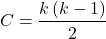
for more on pairwise comparisons, see 10.1 – Compare two independent sample means
For our three group experiment, how many pairwise comparisons can be tested? Therefore,  , and we have
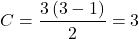
Thus, for our three groups, A, B, and C, there are three possible pairwise comparisons.
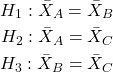
How many pairwise comparisons for a four group experiment? Check your work, you should get  .
The multiple comparison problem
Let’s say that we’re stubborn. We could do many single two-sample t-tests — certainly, your statistical software won’t stop you — this is a situation that calls for statistical reasoning. Here’s why we should not: we will increase the probability of rejecting a null hypothesis when the null hypothesis is true (eg, discussion in Jafari and Ansari-Pour 2019). That is, the chance we will commit a Type I error increases if we do not account for the lack of independence in these sets of pairwise tests evaluated by t-tests. This is multiplicity or the multiple comparison problem.
Review: when we perform a two-sample t-test we are willing to reject a true null hypothesis 5% of the time. This is what is meant by setting the critical probability value (alpha) = 0.05. By “willing” we mean that we know that our conclusions could be wrong because we ar3 working with samples, not the entire population. (Of course at the time, we have no way of actually knowing WHEN we are wrong, but we do want to know how likely we could be wrong!) However, if we compare three population means we have three separate null hypotheses.
HO: one or more of the means are different.
But if we conduct these as separate independent sample t-tests, then we are implicitly making the following null hypothesis statements:
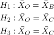
Thus, we have a 5% chance of being wrong for the first hypothesis and/or a 5% chance of being wrong for the second hypothesis and/or a 5% chance of being wrong for the third hypotheses. The chance that we will be wrong for at least one of these hypotheses must now be greater than 5%.
For three separate hypotheses there is a 14% chance of being wrong when we have the probability value for each individual t-test set at α = 0.05. How did we get this result? The point is that these tests are not independent, they are done on the same data set, therefore you can’t simply apply the multiplication probability rule.
Here’s how to figure this: for the set of three hypotheses, the probability of incorrectly rejecting at least one of the null hypotheses is

So, for three t-tests on the same experiment, the Type I error overall tests (experiment-wise) is actually 14% not 5%. It gets worse as the number of combinations (groups and therefore hypotheses) increases. For four groups, Type I error is actually

That’s 26.5%, not 5%.
If we have just five populations means to compare the probability of rejecting a null hypothesis when it is true climbs to 60%! How did this happen? The probability or correctly rejecting all of them is now

So, the probability of incorrectly rejecting one test (Type I error) is now

instead of the 5% we think we are testing.
The key argument for why you must use ANOVA to analyze multiple samples instead of a combination of t-tests!! ANOVA guarantees that the overall error rate is the specified 5%.
Why is the Type I error not 5% for each test? Because we conducted ONE experiment, we can conduct only ONE test (we could be right, we could be wrong 5% of the time). If we conduct the experiment over again, on new subjects, each time resulting in new and therefore independent data sets, then Type I error = 5% for each of these independent experiments.
Now, I hope I have introduced you to the issue of Type I error at the level of a single comparison and the idea of an experiment, holding Type I error-rates at 5% across all hypotheses to be evaluated in an experiment. You may wonder why anyone would make this mistake now. Actually, people make this “mistake” all the time and in some fields like evaluating gene expression for microarray data, this error was the norm, not the exception (see for example discussion of this in Jeanmougin et al 2010).
To conclude, if one does multiple tests on the same experiment, whether it is t-tests or some other test for that matter, then our subsequent tests are related. This is what we mean by independence in statistics — and there are many ways that nonindependence may occur in experimental research. For example, we introduced the concept of pseudoreplication, when observations are treated as if they are independent, but they are not (see Chapter 5.2). The “multiple comparison problem” specifically refers to the lack of independence when all the data set from a single experiment is parsed into lots of separate tests. Philosophically, there must be a logical penalty — and that is reflected in the increase in Type I error.
Clearly something must be done about this!
Corrections to account for the multiple comparisons problem
The family-wise (aka experiment-wise) error rate for multiple comparisons is kept at 5%, and each individual-wise comparison is compared against a more strict (ie, smaller Type I error rate). Put another way, the family-wise error rate is the chance of a number of false positives: making a mistake when we consider many tests simultaneously. The simplest correction for the individual-wise error rate is the Bonferroni correction: test each individual comparison at Type I error equal to  , where C is the number of comparisons. The Šidák correction,
 , and the Holm-Bonferroni method are alternatives with reportedly better statistical properties (eg, reduced Type II error rates; Ludbrook 1998, Sauder and DeMars 2019).
ANOVA is a solution
One possible solution for getting the correct experiment-wise error rate: adjust for differences in probability for multiple comparisons with the t-test. We used post-hoc tests presented above: you could evaluate the tests after accounting for the change in Type I error. This is what is done in many cases. For example, in genomics. In the early days of gene expression profiling by microarray, it was common to see researchers conduct t-tests for each gene. Since microarrays can have thousands of genes represented on the chip, then these researchers were conducting thousands of t-tests, arranging the t-tests by P-value and counting the number of P-values less than 5% and declaring that the differences were statistically significant.
This error didn’t stand long, and there are now many options available to researchers to handle the “multiple comparisons” problem (some probably better than others, research on this very much an ongoing endeavor in biostatistics). The Bonferroni correction was an available solution, largely replaced by the Holm (aka Holm-Bonferroni) method (Holm 1979). Recall that the Bonferroni correction judged individual p-values statistically significant only if they were less than , where, again, α is the family-wise error rate (eg, α = 5%) and C was the number of comparisons. The Holm method orders the C p-values from lowest to highest rank. The method then evaluates lowest p-value, if less than , then reject hypothesis for that comparison. Proceed to next p-value, if less than , then reject hypothesis for that comparison, and so on until no more comparisons are less than .
A MUCH better alternative is to perform a single analysis that takes the multiple-comparisons problem into account: Single Factor ANOVA, also called the one-way ANOVA, plus the post-hoc tests with error correction. We introduce one-way ANOVA in the next section. Post-hoc tests are discussed in Chapter 12.6.
Questions
- You should be able to define and distinguish how Bonferoni correction, Dunnett’s test, and Tukey’s test methods protect against inflation of Type I error.
- What will be the experiment-wise error rate for an experiment in which there are only two treatment groups?
- Experiment-wise error rate may also be called _______________ error rate.
- List and compare the three described posthoc approaches to correct for multiple comparison problem,
- Glycophosphate-tolerant soybean is the number one GMO (genetically modified organism) crop plant worldwide. Glycophosphate is the chief active ingredient in Roundup, the most widely used herbicide. A recent paper examined “food quality” of the nutrient and elemental composition of plants drawn from fields which grow soy by organic methods (no herbicides or pesticides) and GMO plants subject to herbicides and pesticides. A total of 28 individual t-tests were used to compare the treatment groups for different levels of nutrients and elements (eg, vitamins, amino acids, etc.,); the authors concluded that 10 of these t-tests were statistically significant at Type I error rate of 5%. Discuss the approach to statistical inference by the authors of this report; include correct use of the terms experiment-wise and individual-wise in your response and suggest an alternative testing approach if it is appropriate in your view.
- In Chapter 4.2 we introduced a data set from an experiment. The experiment looked at DNA damage quantified by measuring qualities in a Comet Assay including the Tail length, the percent of DNA in the tail, and olive moment. The data set is copied to end of this page. In the next chapter I’ll ask you to conduct the ANOVA on this experiment. For now, answer the following questions.
a. What is the response variable? Defend your choice(s).
b. Why is this an ANOVA problem? Include as part of your explanation a statement of the null hypothesis.
Quiz Chapter 12.1
The need for ANOVA
Data used in this page
comet assay dataset
| Treatment | Tail | TailPercent | OliveMoment* |
|---|---|---|---|
| Copper-Hazel | 10 | 9.7732 | 2.1501 |
| Copper-Hazel | 6 | 4.8381 | 0.9676 |
| Copper-Hazel | 6 | 3.981 | 0.836 |
| Copper-Hazel | 16 | 12.0911 | 2.9019 |
| Copper-Hazel | 20 | 15.3543 | 3.9921 |
| Copper-Hazel | 33 | 33.5207 | 10.7266 |
| Copper-Hazel | 13 | 13.0936 | 2.8806 |
| Copper-Hazel | 17 | 26.8697 | 4.5679 |
| Copper-Hazel | 30 | 53.8844 | 10.238 |
| Copper-Hazel | 19 | 14.983 | 3.7458 |
| Copper | 11 | 10.5293 | 2.1059 |
| Copper | 13 | 12.5298 | 2.506 |
| Copper | 27 | 38.7357 | 6.9724 |
| Copper | 10 | 10.0238 | 1.9045 |
| Copper | 12 | 12.8428 | 2.5686 |
| Copper | 22 | 32.9746 | 5.2759 |
| Copper | 14 | 13.7666 | 2.6157 |
| Copper | 15 | 18.2663 | 3.8359 |
| Copper | 7 | 10.2393 | 1.9455 |
| Copper | 29 | 22.6612 | 7.9314 |
| Hazel | 8 | 5.6897 | 1.3086 |
| Hazel | 15 | 23.3931 | 2.8072 |
| Hazel | 5 | 2.7021 | 0.5674 |
| Hazel | 16 | 22.519 | 3.1527 |
| Hazel | 3 | 1.9354 | 0.271 |
| Hazel | 10 | 5.6947 | 1.3098 |
| Hazel | 2 | 1.4199 | 0.2272 |
| Hazel | 20 | 29.9353 | 4.4903 |
| Hazel | 6 | 3.357 | 0.6714 |
| Hazel | 3 | 1.2528 | 0.2506 |
Tail refers to length of the comet tail, TailPercent is percent DNA damage in tail, and OliveMoment refers to Olive's (1990), defined as the fraction of DNA in the tail multiplied by tail length
Chapter 12 contents
11.2 – Prospective and retrospective power
Introduction
Statistical power is defined as p = 1 – β. The power of a test is the probability of rejecting a Null Hypothesis when it is false. There is a relationship between Type I error and Type II error. We want β to be Large BUT β is generally not known when we are performing the statistical test. We do know that α is inversely related to β. The smaller the α value we use to Reject the Null Hypothesis the MORE likely we will accept a FALSE Null Hypothesis. If we make α very small (one in a billion) then there would be a very HIGH chance of accepting α Null Hypothesis when it is false (β is high). Note that this is the same discussion that we had about sensitivity of an assay test and the specificity of that assay. If we increase sensitivity of the assay such that we approach 100% detection of the true positives will be detected, we necessarily will increase the number of false positives. The BEST way to reduce both Type I and Type II statistical errors is to INCREASE the sample size!
Power of any statistical test (Z test, T-test, one-way ANOVA…) can be determined BEFORE the experiment is done and data are gathered or AFTER an experiment is completed (Cohen 1992). For now, here’s our first real taste of experimental design — we can evaluate how we can make an experiment to test a particular hypothesis.
Prospective power analysis
Good experimental design should include considerations of power. The design will determine the size of the effect your experiment will be able to detect and the probability of correctly rejecting the null hypothesis. In large part, this will involve decisions of sample size and ways to reduce error variance. Moreover, one needs to decide ahead of time, just how large of an effect does the experiment need to detect??? A one-gram change in body mass before and after a diet treatment is of no concern whatsoever if your study subjects are African elephants, but may be a very large effect for a study of shrews!
Retrospective power analysis
Power analysis can also be done after a test has been conducted and the null hypothesis failed to be rejected. One interpretation that might follow from a retrospective power analysis is that, if the study had low power, the lack of statistical significance could be viewed merely the result of low sample size. However, as forcefully argued Hoenig and Heisey (2001) (see also Colegrave and Ruxton 2003), retrospective or posthoc power tests provide no more information than does the p-value and therefore are redundant. At worse, retrospective power analysis can be misleading as to how well it predicts true power, ie, biologically meaningful differences between different treatment groups (Zhang et al., 2019).
Prospective power is more than effect size between groups
Large effect size, ie, large differences between groups, is not necessarily evidence of important biological differences. The concept of power has limits (Hoenig and Heisey 2001 Yuan and Maxwell 2005). On the other hand, small effect sizes can be important differences, especially if the treatment is difficult or expensive. We work through this conclusion with an example, but emphasize here that providing confidence intervals for the effect size (Colegrave and Ruxton 2003). Suppose the null hypothesis was not rejected from a two sample independent t-test conducted on the test of differences in plant height between two samples of `ohi’a found at different elevations. Was there really no difference or was the sample size in the study simply too small to detect the real and important difference between the samples? By conducting a power analysis, one can determine if a slight increase in sample size would have yielded a statistically significant difference, or it may suggest that the effect size is small enough not to warrant further attention.
R code
Three options for conducting power analysis in R are provided in section 11.5
Questions
- Assuming that a study was done by randomly sampling from a population, and the the primary outcome is found not statistically different with p-value 0.13 between placebo and treatment groups, what can be gained made from a retrospective power analysis?
Quiz Chapter 11.2
Prospective and retrospective power
Chapter 11 contents
- Introduction
- What is Statistical Power?
- Prospective and retrospective power
- Factors influencing statistical power
- Two sample effect size
- Power analysis in R
- References and suggested readings
11.1 – What is Statistical Power?
Introduction
Simply put, the power of a statistical test asks the question: do we have enough data to warrant a scientific conclusion, not just a statistical inference. From the NHST approach to statistics, we define two conditions in our analyses, a null hypothesis, HO, and the alternative hypothesis, HA. By now you should have a working definition of HO and HA (Chapter 8.1). For the two-sided case (Chapter 8.4), HO would be no statistical difference between two sample means, whereas for HA, there was a difference between two sample means. Similarly, for one-sided cases, HO would be one sample mean greater (less) than or equal to the second sample mean, whereas for HA, one sample mean is less (greater) than the second mean. Together, these two hypotheses cover all possible outcomes of our experiment!
However, when conducting an experiment to test the null hypothesis four, not two outcomes are possible with respect to “truth” (Table 1), which we introduced first in our Risk analysis chapter and again when we introduced statistical inference.
Table 1. Possible outcomes of an experiment
| In the population, Ho was really… | |||
| True | False | ||
| Inference: | Fail to reject Ho | Correct decision
p = 1 – α |
Type II error
p = β |
| Reject Ho | Type I error
p = α |
Correct decision
p = 1 – β |
|
We introduced false positives and false negatives in our discussion of risk analysis, and now generalize these concepts to outcomes of any experiment.
(1) We do not reject the null hypothesis, we state that we are 95% (P = 1 – α) confident that we’ve made the correct decision, and in fact, that is the true situation (“correct decision”). As before this is a true positive.
For example, mean acetylsalicylic acid concentration in a sample of 200 mg, brand-name aspirin tablets really is the same as generic aspirin.
(2) We reject the null hypothesis, we state there is a 5% chance that we could be wrong (P = 1 – β), and in fact, that is the true situation (“correct decision”). As before this is a true negative.
For example, ephedrine really does raise heart rates in people who have taken the stimulant compared to those who have taken a placebo.
Two additional possible outcomes to an experiment
The other two possible outcomes are not desirable but may occur because we are making inferences about populations from limited information (we conduct tests on samples) and because of random chance influencing our measure.
(3) We do not reject the null hypothesis, but in fact, there was a true difference between the two groups and we have therefore committed a Type II error. As before this is a false negative.
(4) We reject the null hypothesis, but in fact, there was no actual difference between the two groups and we have therefore committed a Type I error. As before this is a false positive.
What can we do about these two possible undesirable outcomes?
We set our Type I error rate α, and, therefore our Type II error rate β before we conduct any tests, and these error rates cover the possibility that we may incorrectly conclude that the null hypothesis is false (α), or we may incorrectly conclude that the null hypothesis is true (β). When might these events happen?
The power of a statistical test is the probability that the test will reject the null hypothesis when the alternative hypothesis is true.
A type I error is committed, by chance alone, when our sample is accidentally obtained from the tail of the distribution, thus our sample appears to be different from the population… Below, we have a possible case that, by chance alone, we could be getting all of our subjects from one end of the distribution (Fig 1).
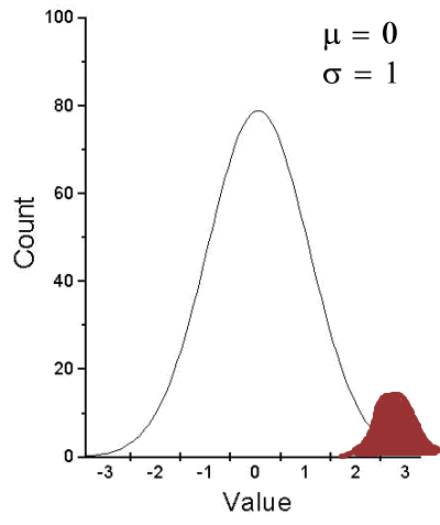
Figure 1. Population sampling from tail of distribution.
We would likely conclude that our sample mean is different (greater) than the population mean.
A type II error is committed, by chance alone, when our sample is between two different population distributions. The implication for our study is drawn in Figure 2. Instead of our sampling drawn from one population, we may have drawn between two very different populations.
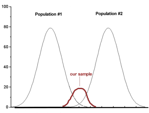
Figure 2. Without us knowing, our sample may come from the extremes of two separate populations.
How did we end up with “the wrong” sample? Recall from our first discussions about Experimental Design how we distinguished between random and haphazard sampling. The key concept was that a program of recruitment of subjects (eg, how to get a sample) must be conducted in such a way that each member of the population has an equal chance of being included in the study. Only then can we be sure that extrinsic factors (things that influence our outcome but are not under our control nor do we study them) are spread over all groups, thus canceling out.
Why do we say we are 95% confident in our estimate (or conclusions)?
(1) Because we can never be 100% certain that by chance alone we haven’t gotten a biased sample (all it takes is a few subjects in some cases to “throw off” our results).
(2) For parametric tests, at least, we assume that we are sampling from a normal population.
Thus, in statistics, we need an additional concept. Not only do we need to know the probability of when we will be wrong (α, β), but we also want to know the probability of when we will be correct when we use a particular statistical test. This latter concept is defined as the power of a test as the probability of correctly rejecting Ho when it is false. Conducting a power analysis before starting the experiment can help answer basic experimental design questions like, how many subjects (experimental units) should my project include? What approximate differences, if any might I expect among the subjects? (Eng 2003; Cohen 1992)
Put another way, power is the likelihood of identifying a significant (important) effect (difference) when one exists. Formally, statistical power is defined as the probability, p = 1 – β, and it is the subject of this chapter.
Questions
- Be able to define and distinguish statistical power and statistical inference.
Quiz Chapter 11.1
What is statistical power
Chapter 11 contents
10.2 – Digging deeper into t-test Plus the Welch test
Introduction
We need to spend some more time with the independent sample t-test; by tearing it apart, we can learn about how parametric tests work in general.
Our assumptions for the independent sample t-test are like the one-sample t-test the data must be continuous and normally distributed (one of our standard assumptions for parametric tests, see Chapter 13). The formula is very similar to the one-sample t-test, except that now we have two sample means and the formula for the standard error (SE) has also changed.

We see that the test statistic t is large if the numerator is large compared to the denominator. Large values of t will be evidence in favor of rejecting the null hypothesis.
The numerator is straightforward: we subtract one sample mean from the other — if there is no difference between the samples, then this difference will be close to zero.
The denominator requires additional discussion. What is it called? It is the pooled standard error of the mean (pooled SEM). Provided the assumption of equal variances holds — an additional standard assumptions for parametric tests, see Chapter 13 — then sample variances estimate the population variance and we can use this information to our advantage to best test the hypothesis about the sample means. In other words, we don’t have to lose a degree of freedom to account for differences in variability for the two groups (see Welch test). More degrees of freedom means more statistical power to test the null hypothesis and at the same time, more confidence that the test is performing to its best.
Lets break down the pooled standard error of the mean in order to see how the assumption of equal variances affects the t-test. We assume that 
Recall that

Now we want a “pooled SE” that is the pooled standard error for both samples. The variance of the difference between the means can be written as
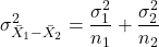
First we need to calculate the pooled variance. where v1 and v2 are degrees of freedom for sample one and sample two, respectively.
Note 1This is just simply a combined formula of the sample variance.
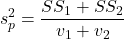
What is SS? The sum of squares , where SS1 and SS2 refer to sum of squares for each of the two groups.
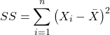
You should recognize SS from your definition of the sample variance, Chapter 3.3.
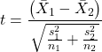
And the standard error for the difference between two means can now be written as So the 2-sample t-test can be written to reflect the pooled sample standard error of the difference between two sample means. We can see how unequal sample size is accommodated by the t-test.
Conducting the test by hand follows the same form as the one-sample t-test. Find the degrees of freedom (DF), but now for each sample.
Finally we evaluate with the critical value in Table (Appendix, Table of Student’s t distribution) and compare the t test statistic against the critical value with the appropriate degrees of freedom.
Because this is the t-test, again, we are assuming that the variances are the same between the two populations (homoscedasticity) and this allows us to pool the variance. As it turns out, the T-test is not overly sensitive to other deviations from the assumptions, but if the variances are in fact different, then the standard formula may yield incorrect Type I error rates compared to stated probability level (α).
However, it would be poor statistical choice to use a test where there are alternatives. This is why in part that R (Rcmdr) sets as the default for the t-test that variances are unequal! In fact, R does not do a t-test unless you change the default to assume equal variances, which, as we now know, is the t-test.
Welch test
What to do when assumptions to t-test are not met? Many options have been proposed, and Welch’s approximate t is a good alternative to the two-sample t-test — it would be appropriate if the normal assumption still held.
The degrees of freedom for the Welch’s test are now
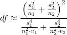
Note 2: The Welch test removes the pooled estimate of the standard error, replaces with both variance estimates directly.
As a default option, R and Rcmdr uses a variation of Welch’s test when you select to do the t-test without making the assumption of equal variance (Fig 1).
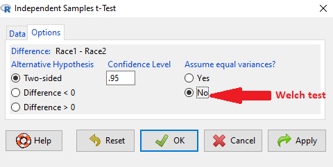
Figure 1. Screenshot Rcmdr t-test options. Default is “No” for Assume equal variances, ie, the Welch test.
The Welch test is not a nonparametric test, it is a different formulation of the t-test.
Justification for beginning with t-test
It’s unlikely that you will need the t-test in today’s research climate. Data sets are large, experiments are complex with multiple variables and samples. Why do we have to consider the t-test, and then a separate test in the case for unequal sample size? I view it as a teaching moment. It makes the general point that ALL statistical tests make assumptions about how the calculations are done and as to the nature of the data set.
This is our first experience with what to do if there is a violation of an assumption of parametric tests (see Chapter 13). Here, the assumption is that the two groups have equal sample size. When they do not, the standard t-test tends to biased estimates. On the other hand, if the assumptions are met, the standard test is the best test because it has more power to do what we intended — that is, it is best at the actual test of the null hypothesis! Take heart — this point is not always appreciated even by scientists (cf. Fagerland 2012).
Note 3: Expert advice will differ here, but you can always calculate the test statistic, even if the assumptions do not hold. The problem, the concern is with the interpretation.
Let’s us approach the problem of violation of assumptions in a couple of ways as an introduction to how, in general, to approach choice of statistical tests.
- Power of a test. Much current statistical research focuses on learning about how a particular statistical test works when assumptions are violated. Thus, in addition to learning what tests are designed to do, we need to consider the effects of violations of assumptions on the performance of the test (namely, is the Type I error at the stated alpha level?). This is a matter of statistical power; power of a test reflects how able the test is to get you the correct result even if assumptions are violated. Often tests perform well if sample sizes are large despite violation of assumptions. We mention without proving that the 2-sample T-test is robust to violations of normality assumption, to requirement for equal sample size, and even to unequal variances. But good experimental design attempts to meet the assumptions because the test does better!
- Alternate forms of some tests are available to handle some aspects of test violations. For example, the simple 2-sample T-test can be modified to accommodate different variances (Welch’s formula). Or you must find a different test (eg, nonparametric tests).
In conclusion, all tests begin with consideration of the assumptions. In some cases we can test our assumptions. For example, we learned about testing the assumption of normal distributions of sample data. We can also test the assumption of equal variances.
Questions
- Consider a clinical trial in which resting blood pressure is recorded on hypertensive subjects at the start of the trial, then 6 weeks after subjects have received daily supplements of flaxseed. Thus, for each subject there are two measures of blood pressure, BEFORE and AFTER.
- Write the null hypothesis
- Write the alternative hypothesis
- Justify why or why not the hypothesis should be two tailed. Explain why or why not an independent sample t-test may be used to compare groups.
Quiz Chapter 10.2
Digging deeper into t-test Plus the Welch test
Chapter 10 contents
- Introduction
- Compare two independent sample means
- Digging deeper into t-test Plus the Welch test
- Paired t-test
- References and suggested reading
10.1 – Compare two independent sample means
Introduction
We introduced the concept of comparing a sample statistic (mean) against a population parameter (Chapter 6.7, Normal deviate) or one-sample t-test against a specified mean (eg, from published data or from theory, Chapter 8.5).
Consider now a basic experimental design, the randomized control trial, or RCT (Fig 1), introduced in Chapter 2.4.
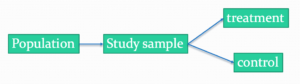
Figure 1. A two group Randomized Control Trial.
Subjects randomly selected from population of interest, then again — random assignment — once recruited into one of two treatment groups. Importantly, subjects belong to one treatment arm only: no subject simultaneously receives the treatment and the control. This is in contrast to the paired design, in which subjects receive both treatments (see Chapter 10.3).
In inferential statistics about an experiment, we are more likely trying to test if sample means are different. For example
- two species grown in common garden, do they differ in growth rate?
- human subjects given a new treatment have better outcomes compare to those receiving a control treatment (eg, placebo).
The equivalent null hypothesis is that two samples are pulled from the same population. We write the null hypothesis as

and the corresponding alternative hypothesis, HA, then must be

Question: Is this a one tailed or two-tailed hypothesis?
Answer: Two-tailed (review Chapter 8.4)
Note 1: In this day and age, there’s really no compelling reason to learn the t-test. First, it is just a special case of the one-way ANOVA, therefore, it’s a special case of the general linear model. Struggling to learn R commands? Well, one solution would be just to learn the general linear model approach — the R function lm() (OK — don’t get too excited — lm() has many options and details). Second, few experiments or observational studies are likely to have only two groups; thus, the temptation to carry out a series of t-tests, taking all groups two at a time, or “pairwise,” while tempting, actually violates a whole bunch of basic statistical rules (discussed in Chapter 12.1). It will also make statisticians go crazy when they see it. That said, if your experiment has but two groups, then by all means, the t-test is a choice. The t-test is also a statistical test that you have likely already used before so we present the discussion here to build on what you may already have learned. We also present the independent t-test as a vehicle.
Worked example
We introduce the two-sample t-test, or better, the independent sample t-test.

where the numerator is the difference between the two sample means and the denominator is the standard error of the differences between the two groups standard errors. The formula for
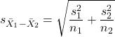
The choice of independent sample over two-sample is best because it emphasizes that the two groups (the two samples), must be comprise of independent sampling units. This is a pretty straight-forward requirement; you have randomly assigned twenty individuals to two groups, a control group (n = 10) and a treatment group (n = 10). Individuals are either in the control group or they are in the treatment group — they cannot simultaneously appear in both groups.
We will work our way through this test by example. For starters, let’s use the same lizard dataset (see Example data set, below), four body mass recordings (grams) each for house geckos (Hemidactylus frenatus, Fig 2) and the Carolina anole (Anolis carolensis, Fig 3), two of many lizard species introduced to Hawaiʻi.

Figure 2. Male Hemidactylus frenatus, central Oahu, M. Dohm.

Figure 3. Male Anolis carolinensis, ʻAkaka Falls, Big Island of Hawaiʻi, M. Dohm.
Example data set
Geckos: 3.186, 2.427, 4.031, 1.995

Anoles: 5.515, 5.659, 6.739, 3.184
Question: How would you go about creating a data frame with the values in long form (stacked worksheet), including a label variable and the body mass?
Note 2: The independent sample t-test in Rcmdr requires a stacked worksheet and not in unstacked worksheet two columns implied by the above pseudo-code. If you need help with worksheet format, then see Part07 in Mike’s Workbook for Biostatistics.
Answer: At the R prompt, type
Geckos <- c(3.186, 2.427, 4.031, 1.995); Anoles = c(5.515, 5.659, 6.739, 3.184) #create two vectors
bmass <- c(Geckos, Anoles)    #combine the two vectors into a single vector holding all of the body mass records
species <- c("gecko", "gecko", "gecko", "gecko", "anole", "anole", "anole", "anole")   #create your label variable
lizards <- data.frame(species, bmass)  #create your data frame
lizards   #print your data frame  species bmass
1   gecko 3.186
2   gecko 2.427
3   gecko 4.031
4   gecko 1.995
5   anole 5.515
6   anole 5.659
7   anole 6.739
8   anole 3.184
Note also that you can enter data into the Data editor by creating the data frame first then adding values. To edit the data frame “lizards” type fix(lizards) at the R prompt, then close the data frame when you have added or changed values as needed.
As always, begin with an exploration of the data, including a graph (Fig 4).
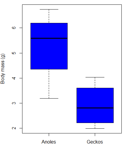
Figure 4. Box plot of lizard body mass.
We can see already that there’s greater spread of data for the Anoles compared to the Geckos, but the median values differ. Small sample sizes can be a problem for analyses as we can only have reduced confidence in our conclusions. However, we press on for the sake of demonstration.
Let’s test the null hypothesis, H0, ie, the two species of lizards have the same mean body mass.
Rcmdr: Statistics → Means → Independent-samples t-test…
In this next image I posted the Rcmdr menu popup for the Independent Samples t-test (Fig 5). Later versions of Rcmdr split the settings for this command into two tabs; the first tab allows for the selection of the variables and setting the hypotheses whereas the second tab, labeled Options, permits additional choices. The default selections need your attention: to actually conduct the t-test you need to answer “No” to the question, “Assume equal variance?” (Fig 6).
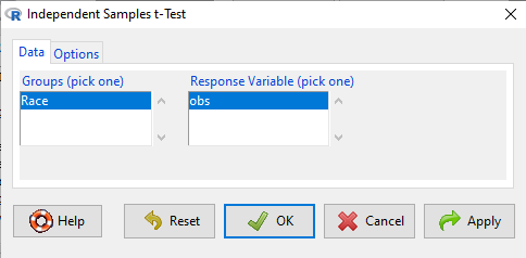
Figure 5. Rcmdr menu for Independent sample t-test.
Select the Options tab (Fig 6) to select null hypothesis and to select the t-test and not the Welch-test (which is the default, ie, No to the prompt “Assume equal variances?”).
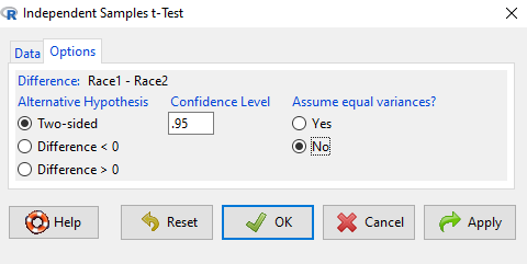
Figure 6. Rcmdr Options menu for Independent sample t-test.
Let’s look at the results and break down the parts of the test.
t.test(Body.mass~Lizard, alternative='two.sided', conf.level=.95,
+ var.equal=TRUE, data=lizards)

Two Sample t-test

data: Body.mass by Lizard
t = 2.7117, df = 6, p-value = 0.03503
alternative hypothesis: true difference in means is not equal to 0
95 percent confidence interval:
0.2308685 4.4981315
sample estimates:
mean in group Anolis mean in group Gecko
5.27425 2.90975
Consider the R session output above and answer the following questions.
Questions for the worked example
- Which lizard group had the greater mean value, Anolis or Gecko?
- What are the assumptions necessary for you to use the independent sample t-test?
- What does “two-sided” mean?
- What was the null hypothesis?
- Was this a one-tailed or two-tailed test of the null hypothesis?
- What is the value of the test statistic?
- How many degrees of freedom?
- What is the critical value for this test?
- What is the value of the lower limit of the 95% confidence interval?
- What is the value of the lower limit of the 99% confidence interval?
- True or False. If the null hypothesis is accepted, then zero is a value included in the 95% confidence interval.
- Do you accept the null hypothesis? Explain your selection.
Try another example
DNA damage, changes in the chemical structure of nucleotide bases or breakage of the DNA chains, occurs in cells under many circumstances. The comet assay, or single-cell gel electrophoresis, is one method for visualizing and measuring DNA strand breaks in cells. Exposed cells are mixed with a low-melting temperature agarose and placed onto a microscope slide. The cells are then lysed with an alkaline detergent and high salts. When current is applied across the slide, undamaged DNA remains in the nucleus, whereas damaged DNA extends towards the anode to form a comet-like tail, with imaging assisted by including a fluorescent dye like Sybr-Green. Examples of comets are shown below (Fig 7).
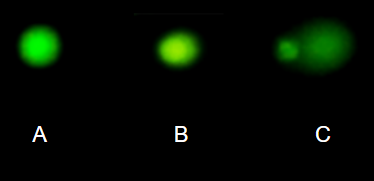
Figure 7. Comet examples. A Intact cell, no DNA damage, B Cell with some DNA damage, a slight tail to the right is evident, C Cell with significant DNA damage, a large tail is evident. M. Dohm.
In an experiment, immortalized lung epithelial cells were exposed to dilute copper solutions for 30 minutes then washed with PBS. The comet assay was applied to these cells and for comparison, to cells without copper exposure but otherwise treated the same way (controls). The data are available at the bottom of this page (scroll down or click here).
Again, you should begin all analyses with an exploration of the data, including a graph (Fig 8).
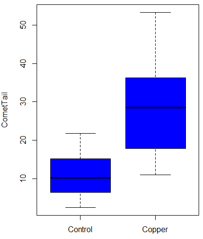
Figure 8. Boxplot of comet tail lengths for cells with and without (control) exposure to copper in the cell medium for 30 minutes.
Let’s look at the R output for the t-test analysis.
    Two Sample t-test

data:  CometTail by Treatment
t = -5.8502, df = 38, p-value = 9.139e-07
alternative hypothesis: true difference in means is not equal to 0
95 percent confidence interval:
 -22.39865 -10.88213
sample estimates:
mean in group Control  mean in group Copper
             11.14533              27.78571
Consider the R session output above and answer the following questions.
Questions for Comet assay data set
- Which cell group had the greater mean value, Copper-exposed or Control-exposed cells?
- What are the assumptions necessary for you to use the independent sample t-test?
- What does “two-sided” mean?
- What was the null hypothesis?
- Was this a one-tailed or two-tailed test of the null hypothesis?
- What is the value of the test statistic?
- How many degrees of freedom?
- What is the critical value for this test?
- What is the value of the lower limit of the 95% confidence interval?
- What is the value of the lower limit of the 99% confidence interval?
- True or False. If the null hypothesis is accepted, then zero is a value included in the 95% confidence interval.
- Do you accept the null hypothesis? Explain your selection.
T test from summary statistics
In some cases you may only have to summary statistics for data, eg, the means and the standard deviations. We can use the equations of the t test to write a simple formula, where the user provides the known means, standard deviations, and sample size. For example, create a simple function with readline for user input.
myTtest <- function() {
   mnx <- as.numeric(readline(prompt="Enter mean of x: "))
   stdevx <- as.numeric(readline(prompt="Enter sd of x: "))
   nx <- as.numeric(readline(prompt="Enter n of x: "))
   mny <- as.numeric(readline(prompt="Enter mean of y: "))
   stdevy <- as.numeric(readline("Enter sd of y: "))
   ny <- as.numeric(readline(prompt="Enter n of y: "))
   myTvalue <- abs(((mnx-mny)-0)/sqrt(((stdevx^2)/nx)+(stdevy^2)/ny))
   myDF <- as.integer(nx+ny-2)
   myPvalue <- pt(myTvalue,myDF,lower.tail=FALSE)*2
   myResults <- c(myTvalue, myDF, myPvalue)
   report <- c("T-test: ", "df: ", "two-tailed p-value: ")
   cat(sprintf("%s %3.3f, ", report, myResults))
}
then run the function by typing myTest() at the R prompt and entering the means, standard deviations, and sample size when prompted.
myTtest()
Enter mean of x: 2.91
Enter sd of x: .895
Enter n of x: 4
Enter mean of y: 5.27
Enter sd of y: 1.497
Enter n of y: 4
T-test: 2.706, df: 6.000, two-tailed p-value: 0.035
P-values from confidence intervals
While we expect certain reporting criteria for published, it is not uncommon that one or more elements are missing. For example, while means plus or minus standard deviations for two groups may be reported, the confidence interval of the difference may not be reported, or, an inexact p-value is reported like “< 0.05,” but we “need” an exact p-value for our meta-analysis. A little math, and these missing statistics can be calculated.
We can use the lizard study as an example; while all of the expected elements were reported, including the p-value (0.03503), let’s say the p value was reported as “statistically significant at p < 0.05.”
We need
lower and upper confidence intervals: 0.2309 and 4.498, respectively.
critical value from t distribution, df = 6 (2 tailed, therefore 0.05/2). A little R code we have:

the standard error, which can be calculated as 
and then the p-value, 
which is pretty close to the result from R (p = 0.03503). The difference is likely due to the small sample size.
Questions
- Don’t forget to work through the Questions for the Comet tail data set (scroll up or click here).
- Microsoft Excel, LibreOffice Calc, and Google sheets spreadsheet software all include t-test functions and return the p-value. Consider two variables big (100, 110, 120, 100, 110, 210, 200) and small (0,1,1,2,0,1,0). (Note — these two groups are obviously very different, calculating a t-test on their difference is silly, just for this question.) If formatting is set to the default two decimal places for Number cell category, the p-value will return as “0.00.” How should you report the p-value in this case?
Quiz Chapter 10.1
Compare two independent sample means
Comet assay data set
| Treatment | CometTail |
| Control | 17.856139 |
| Control | 16.52125 |
| Control | 14.925449 |
| Control | 14.029174 |
| Control | 13.332945 |
| Control | 8.811185 |
| Control | 14.701654 |
| Control | 9.261025 |
| Control | 21.779311 |
| Control | 6.180284 |
| Control | 9.201752 |
| Control | 5.54472 |
| Control | 6.717885 |
| Control | 2.625092 |
| Control | 7.191583 |
| Control | 5.392866 |
| Control | 11.284813 |
| Control | 15.441254 |
| Control | 17.857176 |
| Control | 4.250956 |
| Copper | 53.214287 |
| Copper | 38.92857 |
| Copper | 18.928572 |
| Copper | 30 |
| Copper | 28.928572 |
| Copper | 15.357142 |
| Copper | 17.857143 |
| Copper | 17.5 |
| Copper | 21.071428 |
| Copper | 29.285715 |
| Copper | 28.214285 |
| Copper | 16.785715 |
| Copper | 21.071428 |
| Copper | 37.5 |
| Copper | 38.214287 |
| Copper | 17.857143 |
| Copper | 29.642857 |
| Copper | 11.071428 |
| Copper | 35 |
| Copper | 49.285713 |
Chapter 10 contents
- Introduction
- Compare two independent sample means
- Digging deeper into t-test Plus the Welch test
- Paired t-test
- References and suggested reading
9.1 – Chi-square test: Goodness of fit
Introduction
We ask about the “fit” of our data against predictions from theory, or from rules that set our expectations for the frequency of particular outcomes drawn from outside the experiment. Three examples to illustrate goodness of fit, GOF,  , A, B, and C follow.
A. For example, for a toss of a coin, we expect heads to show up 50% of the time. Out of 120 tosses of a fair coin, we expect 60 heads, 60 tails. Thus, our null hypothesis would be that heads would appear 50% of the time. If we observe 70 heads in an experiment of coin tossing, is this a significantly large enough discrepancy to reject the null hypothesis?
B. For example, simple Mendelian genetics makes predictions about how often we should expect particular combinations of phenotypes in the offspring when the phenotype is controlled by one gene, with 2 alleles and a particular kind of dominance.
For example, for a one locus, two allele system (one gene, two different copies like R and r) with complete dominance, we expect the phenotypic (what you see) ratio will be 3:1 (or  round,
 wrinkle). Our null hypothesis would be that pea shape will obey Mendelian ratios (3:1). Mendel’s round versus wrinkled peas (RR or Rr genotypes give round peas, only rr results in wrinkled peas).
Thus, out of 100 individuals, we would expect 75 round and 25 wrinkled. If we observe 84 round and 16 wrinkled, is this a significantly large enough discrepancy to reject the null hypothesis?
C. For yet another example, in population genetics, we can ask whether genotypic frequencies (how often a particular copy of a gene appears in a population) follow expectations from Hardy-Weinberg model (the null hypothesis would be that they do).
This is a common test one might perform on DNA or protein data from electrophoresis analysis. Hardy-Weinberg is a simple quadratic expansion:
If p = allele frequency of the first copy, and q = allele frequency of the second copy, then p + q = 1,
Given the allele frequencies, then genotypic frequencies would be given by 1 = p2 + 2pq + q2.
Deviations from Hardy-Weinberg expectations may indicate a number of possible causes of allele change (including natural selection, genetic drift, migration).
Thus, if a gene has two alleles,  and
 , with the frequency for ,
 and for ,
 (equivalently q = 1 – p) in the population, then we would expect 36
 , 16
 , and 48
 individuals. (Nothing changes if we represent the alleles as A and a, or some other system, eg, dominance/recessive.)
Question. If we observe the following genotypes: 45 individuals, 34 individuals, and 21 individuals, is this a significantly large enough discrepancy to reject the null hypothesis?
Table 1. Summary of our Hardy Weinberg question
| Genotype | Expected | Observed | O – E |
| aa | 70 | 45 | -25 |
| aa’ | 27 | 34 | 7 |
| a’a’ | 3 | 21 | 18 |
| sum | 100 | 100 | 0 |
Recall from your genetics class that we can get the allele frequency values from the genotype values, eg,
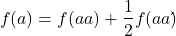
We call these chi-square tests, tests of goodness of fit. Because we have some theory, in this case Mendelian genetics, or guidance, separate from the study itself, to help us calculate expected values in a chi-square test.
Note 1: The idea of fit in statistics can be reframed as how well does a particular statistical model fit the observed data. A good fit can be summarized by accounting for the differences between the observed values and the comparable values predicted by the model.
Note also for our coin toss example, goodness of fit isn’t exactly proper terminology — afterall the test is equal probability of the two outcomes, not whether we have match between an observed distribution and an expected distribution (true statement if we add “follows a binomial distribution”).
 goodness of fit
For k groups, the equation for the chi-square test may be written as
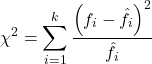
where fi is the frequency (count) observed (in class i) and fi<hat> is the frequency (count) expected if the null hypothesis is true, sum over all k groups. Alternatively, here is a format for the same equation that may be more familiar to you… ?
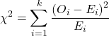
where Oi is the frequency (count) observed (in class i) and Ei is the frequency (count) expected if the null hypothesis is true.
The degrees of freedom, df, for the GOF are simply the number of categories minus one, k – 1.
Explaining GOF
Why am I using the phrase “goodness of fit?” This concept has broad use in statistics, but in general it applies when we ask how well a statistical model fits the observed data.
At least for the chi-square test it is simple to see how the test statistic increases from zero as the agreement between observed data and expected data depart, where zero would be the case in which all observed values for the categories exactly match the expected values.
The goodness of fit test is designed to evaluate whether or not your data agree with a theoretical expectation (there are additional ways to think about this test, but this is a good place to start). Let’s take our time here and work with an example. The other type of chi-square problem or experiment is one for the many types of experiments in which the response variable is discrete, just like in the GOF case, but we have no theory to guide us in deciding how to obtain the expected values. We can use the data themselves to calculate expected values, and we say that the test is “contingent” upon the data, hence these types of chi-square tests are called contingency tables.
You may be a little concerned at this point that there are two kinds of chi-square problems, goodness of fit and contingency tables. We’ll deal directly with contingency tables in the next section, but for now, I wanted to make a few generalizations.
- Both goodness of fit and contingency tables use the same chi-square equation and analysis. They differ in how the degrees of freedom are calculated.
- Thus, what all chi-square problems have in common, whether goodness of fit or contingency table problems
- You must identify what types of data are appropriate for this statistical procedure? Categorical (nominal data type).
- As always, a clear description of the hypotheses being examined.
For goodness of fit chi-square test, the most important type of hypothesis is called a Null Hypothesis: In most cases the Null Hypothesis (HO) is “no difference” “no effect”…. If HO is concluded to be false (rejected), then an alternative hypothesis (HA) will be assumed to be true. Both are specified before tests are conducted. All possible outcomes are accounted for by the two hypotheses.
From above, we have
- A. HO: Fifty out of 100 tosses will result in heads.
- HA: Heads will not appear 50 times out of 100.
- B. HO: Pea shape will equal Mendelian ratios (3:1).
- HA: Pea shape will not equal Mendelian ratios (3:1).
- C. HO: Genotypic frequencies will equal Hardy-Weinberg expectations.
- HA: Genotypic frequencies will not equal Hardy-Weinberg expectations
Assumptions: In order to use the chi-square, there must be two or more categories. Each observation must be in one and only one category. If some of the observations are truly halfway between two categories then you must make a new category (eg, low, middle, high) or use another statistical procedure. Additionally, your expected values are required to be integers, not ratio. The number of observed and the number of expected must sum to the same total.
The chi-square test is a good example of such tests, and we will encounter other examples too. Another common goodness of fit is the coefficient of determination, which will be introduced in linear regression sections (see Chapter 17.7 – Regression model fit). Still other examples are the likelihood ratio test (LRT), Akaike Information Criterion (AIC), and Bayesian Information Criterion (BIC), which are all used to assess fit of models to data. (See Graffelman and Weir [2018] for how to use AIC in the context of testing for Hardy Weinberg equilibrium.)
The likelihood ratio test is used to compare the goodness of fit of two hierarchically nested models to determine if a more complex model provides a significantly better fit to the data. It does this by forming a ratio of the likelihood of the data under the two models (the simpler “null” model and the more complex “alternative” model). A small ratio suggests the simpler model is a poor fit, while a value close to one indicates the added complexity is not statistically significant. AIC (and BIC) is a measure of relative fit — it balances goodness of fit and model complexity: A lower AIC suggests a better model by finding the optimal trade-off between fitting the data well and keeping the model simple. A model that is too complex will have a higher AIC than a simpler model with a nearly as good fit.
We use LRT, AIC and BIC when we talk about selecting best regression models (see Chapter 17.7 – Regression model fit). However, as we discuss the concept of comparing models, we need to distinguish between the concept of model choice — methods used to select a best model from competing options and estimating the “goodness of fit” of a single model.
How well does data fit the prediction?
Frequentist approach interprets the test as, how well does the data fit the null hypothesis,  ? When you compare data against a theoretical distribution (eg, Mendel’s hypothesis predicts the distribution of progeny phenotypes for a particular genetic system), you test the fit of the data against the model’s predictions (expectations). Recall that the Bayesian approach asks how well does the model fit the data?
Table 2. A. 120 tosses of a coin, we count heads 70/120 tosses.
| Expected | Observed | |
| Heads | 60 | 70 |
| Tails | 60 | 50 |
| n | 120 | 120 |

Table 3. B. A possible Mendelian system of inheritance for a one gene, two allele system with complete dominance, observe the phenotypes.
| Expected | Observed | |
| Round | 75 | 84 |
| Wrinkled | 25 | 16 |
| n | 100 | 100 |

Table 4. C. A possible Mendelian system of inheritance for a one gene, two allele system with complete dominance, observe the phenotypes.
| Expected | Observed | |
| p2 | 70 | 45 |
| 2pq | 27 | 34 |
| q2 | 3 | 21 |
| n | 100 | 100 |

For completeness, instead of a goodness of fit test we can treat this problem as a test of independence, a contingency table problem. We’ll discuss contingency tables more in the next section, but or now, we can rearrange our table of observed genotypes for problem C, as a 2X2 table
Table 5. Problem C reported in 2X2 table format.
| Maternal a’ | Paternal a’ | |
| Maternal a | 45 | 17 |
| Paternal a | 17 | 21 |
The contingency table is calculated the same way as the GOF version, but the degrees of freedom are calculated differently: df = number of rows – 1 multiplied by the number of columns – 1.

Thus, for a 2X2 table the df are always equal to 1.
Note that the chi-square value itself says nothing about how any discrepancy between expectation and observed genotype frequencies come about. Therefore, one can rearrange the equation to make clear where deviance from equilibrium, D, occur for the heterozygote (het). We have

where D2 is equal to
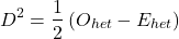
φ coefficient
The chi-square test statistic and its inference tells you about the significance of the association, but not the strength or effect size of the association. Not surprisingly, Pearson (1904) came up with a statistic to quantify the strength of association between two binary variables, now called the φ (phi) coefficient. Like the Pearson product moment correlation, the φ (phi) coefficient takes values from -1 to +1.
Note 2: Pearson termed this statistic the mean square contingency coefficient. Yule (1912) termed it the phi coefficient. The correlation between two binary variables is also called the Mathews Correlation Coefficient or MCC (Mathews 1975), which is a common classification tool in machine learning.
The formula for the absolute value of φ coefficient is

Thus, for A, B, and C examples, φ coefficient was 0.167, 0.190, and 0.771. Thus, only weak associations in examples A and B, but strong association in C. We’ll provide a formula to directly calculate φ coefficient from the cells of the table in 9.2 – Chi-square contingency tables.
Carry out the test and interpret results
What was just calculated? The chi-square, , test statistic.
Just like t-tests, we now want to compare our test statistic against a critical value — calculate degrees of freedom (df = k – 1, k equals the numbers of categories), and set a rejection level, Type I error rate. We typically set the Type I error rate at 5%. A table of critical values for the chi-square test is available in Appendix Table Chi-square critical values.
Obtaining Probability Values for the goodness-of-fit test of the null hypothesis:
As you can see from the equation of the chi-square, a perfect fit between the observed and the expected would be a chi-square of zero. Thus, asking about statistical significance in the chi-square test is the same as asking if your test statistic is significantly greater than zero.
The chi-square distribution is used and the critical values depend on the degrees of freedom. Fortunately for and other statistical procedures we have Tables that will tell us what the probability is of obtaining our results when the null hypothesis is true (in the population).
Here is a portion of the chi-square critical values for probability that your chi-square test statistic is less than the critical value (Fig 1).
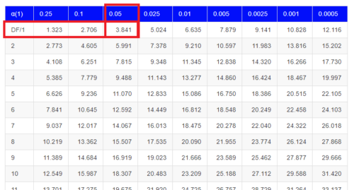
Figure 1. A portion of critical values of the chi-square at alpha 5% for degrees of freedom between 1 and 10. A more inclusive table is provided in the Appendix, Table of Chi-square critical values.
For the first example (A), we have df = 2 – 1 = 1 and we look up the critical value corresponding to the probability in which Type I = 5% are likely to be smaller iff (“if and only if”) the null hypothesis is true. That value is 3.841; our test statistic was 3.330, and therefore smaller than the critical value: so we do not reject the null hypothesis.
Interpolating p-values
How likely is our test statistic value of 3.333 and the null hypothesis was true? (Remember, “true” in this case is a shorthand for our data was sampled from a population in which the HW expectations hold). When I check the table of critical values of the chi-square test for the “exact” p-value, I find that our test statistic value falls between a p-value 0.10 and 0.05 (represented in the table below). We can interpolate
Note 3: Interpolation refers to any method used to estimate a new value from a set of known values. Thus, interpolated values fall between known values. Extrapolation on the other hand refers to methods to estimate new values by extending from a known sequence of values.
Table 6. Interpolated p-value for critical value not reported in chi-square table.
| statistic | p-value |
| 3.841 | 0.05 |
| 3.333 | x |
| 2.706 | 0.10 |
If we assume the change in probability between 2.706 and 3.841 for the chi-square distribution is linear (it’s not, but it’s close), then we can do so simple interpolation.
We set up what we know on the right hand side equal to what we don’t know on the left hand side of the equation,

and solve for x. Then, x is equal to 0.0724
R function pchisq() gives a value of p = 0.0679. Close, but not the same. Of course, you should go with the result from R over interpolation; we mention how to get the approximate p-value by interpolation for completeness, and, in some rare instances, you might need to make the calculation. Interpolating is also a skill used to provide estimates where the researcher needs to estimate (impute) a missing value.
Interpreting p-values
This is a pretty important topic, so much so that we devote an entire section to this very problem — see 8.2 – The controversy over proper hypothesis testing. If you skipped the chapter, but find yourself unsure how to interpret the p-value, then please go back to Ch 8.2. OK, that commercial message, what does it mean to “reject the chi-square null hypothesis?” These types of tests are called goodness of fit in the following sense — if your data agree with the theoretical distribution, then the difference between observed and expected should be very close to zero. If it is exactly zero, then you have a perfect fit. In our coin toss case, if we say that the ratio of heads:tails do not differ significantly from the 50:50 expectation, then we accept the null hypothesis.
You should try the other examples yourself! A hint, the degrees of freedom are one (1) for example B and two (2) for example C.
R code
Printed tables of the critical values from the chi-square distribution, or for any statistical test for that matter are fine, but with your statistical package R and Rcmdr, you have access to the critical value and the p-value of your test statistic simply by asking. Here’s how to get both.
First, let’s get the critical value.
Rcmdr: Distributions → Continuous distributions → Chi-squared distribution → Chi-squared quantiles (Fig 2).
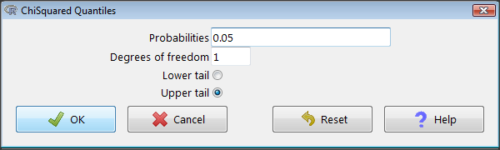
Figure 2. R Commander menu for Chi-squared quantiles.
I entered “0.05” for the probability because that’s my Type I error rate α. Enter “1” for Degrees of freedom, then click “upper tail” because we are interested in obtaining the critical value for α. Here’s R’s response when I clicked “OK.”
qchisq(c(0.05), df=1, lower.tail=FALSE)
[1] 3.841459
Next, let’s get the exact P-value of our test statistic. We had three from three different tests:  for the coin-tossing example,
 for the pea example, and
 for the Hardy-Weinberg example.
Rcmdr: Distributions → Continuous distributions → Chi-squared distribution → Chi-squared probabilities… (Fig 3).
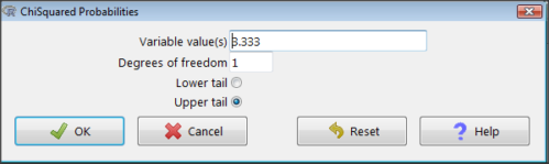
Figure 3. R Commander menu for Chi-squared probabilities.
I entered “3.333” because that is one of the test statistics I want to calculate for probability and “1” for Degrees of freedom because I had k – 1 = 1 df for this problem. Here’s R’s response when I clicked “OK.”
pchisq(c(3.333), df=1, lower.tail=FALSE)
[1] 0.06790291
I repeated this exercise for I got  ; for I got
 .
Nice, right? Saves you from having to interpolate probability values from the chi-square table.
3. How to get the goodness of fit in Rcmdr.
R provides the goodness of fit (the command is chisq.text()), but Rcmdr thus far does not provide a menu option to link to the function. Instead, R Commander provides a menu for contingency tables, which also is a chi-square test, but is used where no theory is available to calculate the expected values (see Chapter 9.2). Thus, for the goodness of fit chi-square, we will need to bypass Rcmdr in favor of the script window. Honestly, other options are as quick or quicker: calculate by hand, use a different software (eg, Microsoft Excel), or many online sites provide JavaScript tools.
So how to get the goodness of fit chi-square while in R? Here’s one way. At the command line, type
chisq.test (c(O1, O2, ... On), p = c(E1, E2, ... En))
where O1, O2, … On are observed counts for category 1, category 2, up to category n, and E1, E2, … En are the expected proportions for each category. For example, consider our Heads/Tails example above (problem A).
In R, we write and submit
chisq.test(c(70,30),p=c(1/2,1/2))
R returns
Chi-squared test for given probabilities.
data: c(70, 30)
X-squared = 16, df = 1, p-value = 0.00006334
Easy enough. But not much detail — details are available with some additions to the R script. I’ll just link you to a nice website that shows how to add to the output so that it looks like the one below.
mike.chi <- chisq.test(c(70,30),p=c(1/2,1/2))
Let’s explore one at time the contents of the results from the chi square function.
names(mike.chi)   #The names function
[1] "statistic" "parameter" "p.value" "method" "data.name" "observed"
[7] "expected" "residuals" "stdres"
Now, call each name in turn.
mike.chi$residuals
[1] 2.828427 -2.828427
mike.chi$obs
[1] 70 30
mike.chi$exp
[1] 50 50
Note 4: “residuals” here simply refers to the difference between observed and expected values. Residuals are an important concept in regression, see Ch17.5
And finally, let’s get the summary output of our statistical test.
mike.chi
Chi-squared test for given probabilities.
data: c(70, 30)
X-squared = 16, df = 1, p-value = 6.334e-05
GOF and spreadsheet apps
Easy enough with R, but it may even easier with other tools. I’ll show you how to do this with spreadsheet apps and with and online at graphpad.com.
Let’s take the pea example above. We had 16 wrinkled, 84 round. We expect 25% wrinkled, 75% round.
Now, with R, we would enter
chisq.test(c(16,80),p=c(1/4,3/4))
and the R output
Chi-squared test for given probabilities
data: c(16, 80)
X-squared = 3.5556, df = 1, p-value = 0.05935
Microsoft Excel and the other spreadsheet programs (Apple Numbers, Google Sheets, LibreOffice Calc) can calculate the goodness of fit directly; they return a P-value only. If the observed data are in cells A1 and A2, and the expected values are in B1 and B2, then use the procedure =CHITEST(A1:A2,B1:B2).
Table 7. A spreadsheet with formula visible.
| A | B | C | D | |
| 1 | 80 | 75 | ||
| 2 | 16 | 25 | =CHITEST(A1:A2,B1:B2) |
The P-value (but not the Chi-square test statistic) is returned. Here’s the output from Calc.
Table 8. Spreadsheet example from Table 7 with calculated P-value.
| A | B | C | D | |
| 1 | 80 | 75 | ||
| 2 | 16 | 25 | 0.058714340077662 |
You can get the critical value from MS Excel (=CHIINV(alpha, df), returns the critical value), and the exact probability for the test statistic =CHIDIST(x,df), where x is your test statistic. Putting it all together, a general spreadsheet template for goodness of fit calculations calculations of test statistic and p-value might look like
Table 9. Spreadsheet template with formula to calculate chi-square goodness of fit on two groups.
| A | B | C | D | E | |
| 1 | f1 | 0.75 | |||
| 2 | f2 | 0.25 | |||
| 3 | N | =SUM(A5,A6) |
|||
| 4 | Obs | Exp | Chi.value | Chi.sqr | |
| 5 | 80 | =B1* |
=((A5-B5)^2)/B5 |
=SUM(C5,C6) |
|
| 6 | 16 | =B2* |
=((A6-B6)^2)/B6 |
=CHIDIST(D5, COUNT(A5:A6-1) |
|
| 7 | |||||
| 8 |
 3
Microsoft Excel can be improved by writing macros, or by including available add-in programs, such as the free PopTools, which is available for Microsoft Windows 32-bit operating systems only.
Another option is to take advantage of the internet — again, many folks have provided java or JavaScript-based statistical routines for educational purposes. Here’s an easy one to use www.graphpad.com.
In most cases, I find the chi-square goodness-of-fit is so simple to calculate by hand that the computer is redundant.
Questions
1. A variety of p-values were reported on this page with no attempt to reflect significant figures or numbers of digits (see Chapter 8.2). Provide proper significant figures and numbers of digits as if these p-values were reported in a science journal.
- 0.0724
- 0.0679
- 0.03766692
- 0.004955794
- 0.00006334
- 6.334e-05
- 0.05935
- 0.058714340077662
2. For a mini bag of M&M candies, you count 4 blue, 2 brown, 1 green, 3 orange, 4 red, and 2 yellow candies.
- What are the expected values for each color?
- Calculate using your favorite spreadsheet app (eg, Numbers, Excel, Google Sheets, LibreOffice Calc)
- Calculate using R (note R will reply with a warning message that the “Chi-squared approximation may be incorrect”; see 9.2 Yates continuity correction)
- Calculate using Quickcalcs at graphpad.com
- Construct a table and compare p-values obtained from the different applications
3. CYP1A2 enzyme involved with metabolism of caffeine. Folks with C at SNP rs762551 have higher enzyme activity than folks with A. Populations differ for the frequency of C. Using R or your favorite spreadsheet application, compare the following populations against global frequency of C is 33% (frequency of A is 67%).
- 286 persons from Northern Sweden: f(C) = 26%, f(A) = 73%
- 4532 Native Hawaiian persons: f(C) = 22%, f(A) = 78%
- 1260 Native American persons: f(C) = 30%, f(A) = 70%
- 8316 Native American persons: f(C) = 36%, f(A) = 64%
- Construct a table and compare p-values obtained for the four populations.
Quiz Chapter 9.1
Chi-square test: Goodness of fit
Chapter 9 contents
8.4 – Tails of a test
Introduction
The basics of statistical inference is to establish the null and alternative hypotheses. Starting with the simplest cases, where there is one sample of observations and the comparison is against a population (theory) mean, how many possible comparisons can be made? The next simplest is the two-sample case, where we have two sets of observations and the comparison is against the two groups. Again, how many total comparisons may be made?
Let , “X bar”, equal the sample mean and  , “mu”, represent the population mean. For sample means, designate groups by a subscript, 1 or 2. We then have Table 1.
Table 1. Possible hypothesis involving two groups
| Comparison | One-same | Two-sample |
| 1. |  |
 |
| 2. |  |
 |
| 3. |  |
 |
| 4. |  |
 |
| 5. |  |
 |
| 6. |  |
 |
Classical statistics classifies inference into null hypothesis, HO, vs. alternative hypotheses, HA, and specifies that we test null hypotheses based on the value of the estimated test statistic (see discussion about critical value and p-value, Chapter 8.2). From the list of six possible comparisons we can divide them into one-tailed and two-tailed differences (Table 1). By “tail” we are referring to the ends or tails of a distribution (Figure 1, Figure 2); where do our results fall on the distribution?
Two-tailed hypotheses: Comparison 1 and comparison 2 in the table above are two-tailed hypotheses. We don’t ask about the direction of any difference (less than or greater than).
Figure 1 shows the “two-tailed” distribution — if our results fall to the left ,  , or to the right
 we reject the null hypothesis (blue regions in the curve). We divide the type I error into two equal halves.
Note 1: It’s a nice trick to shade in regions of the curve. A package tigerstats includes the function pnormGC that simplifies this task.
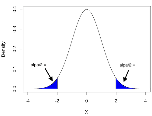
Figure 1. Two-tailed distribution.
RcmdrMisc::plotDistr(x = seq(-4, 4, length.out = 100),
  p = dnorm(seq(-4, 4, length.out = 100)),
  regions = list(c(-Inf, -1.96), c(1.96, Inf)),
  xlab="X", ylab="Density",
  col=c("blue"),
  legend=FALSE)
Figure 2 shows the “one-tailed” distribution — if our alternative hypothesis was that the sample mean was less than the population mean, then our fall to the left,  , for the “lower tail” of the distribution. If, however, our alternative hypothesis was that the sample mean was greater than the population mean, then our region of interest falls to the right,
 . Again, we reject the null hypothesis (blue regions in the curve). Note for one-tailed hypothesis, all Type I error occurs in the one area, not both, so
 (alpha) remains 0.05 over the entire rejection region (Fig 2).
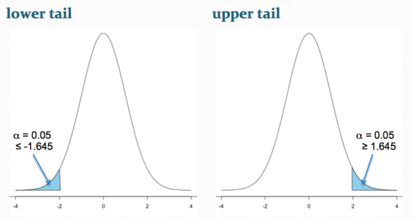
Figure 2. One-tailed distribution, lower tail (left) and upper tail (right).
library(tigerstats)
pnormGC(1.645, region="above", mean=0, sd=1,graph=TRUE)
pnormGC(-1.645, region="below", mean=0, sd=1,graph=TRUE)
One-tailed hypotheses: Comparison 3 through comparison 6 in the table are one-tailed hypotheses. The direction of the difference matters.
Note a simple trick to writing one-tailed hypotheses: first write the alternative hypothesis because the null hypothesis includes all of the other possible outcomes of the test.
Examples
Let’s consider some examples. We learn best by working through cases.
Chemotherapy as an approach to treat cancers owes its origins to the work of Dr Sidney Farber among others in the 1930s and ’40s (DeVita and Chu 2008; Mukherjee 2011). Following up on the observations of others that folic acid (vitamin B9) improved anemia, Dr Farber believed that folic acid might reverse the course of leukemia (Mukherjee 2011). In 1946 he recruited several children with acute lymphoblastic leukemia and injected them with folic acid. Instead of ameliorating their symptoms (eg, white blood cell counts and percentage of abnormal immature white blood cells, called blast cells), treatments accelerated progression of the disease. That’s a scientific euphemism for the reality — the children died sooner in Dr. Faber’s trial than patients not enrolled in his study. He stopped the trials. Clearly, adding folic acid was not a treatment against this leukemia.
Question 1. Do you think these experiments are one sample or two sample? Hint: Is there mention of a control group?
Answer: There’s no mention of a control group, but instead, Dr. Faber would have had plenty of information about the progression of this disease in children. This was a one sample test.
Question 2. What would be a reasonable interpretation of Dr Faber’s alternative hypothesis with respect to percentage of blast cells in patients given folic acid treatment? Your options are
- Folic acid supplementation has an effect on blast counts.
- Folic acid supplementation reduces blast counts.
- Folic acid supplementation increases blast counts.
- Folic acid supplementation has no effect on blast counts.
Answer: At the start of the trials, it is pretty clear that the alternative hypothesis was intended to be a one-tailed test (option 2). Dr. Faber’s alternative hypothesis clearly was that he believed that addition of folic acid would reduce blast cell counts. However, that they stopped the trials shows that they recognized that the converse had occurred, that blast counts increased; this means that, from a statistician’s point of view, Dr Faber’s team was testing a two-sided hypothesis (option 1).
Another example.
Dr Farber reasoned that if folic acid accelerated leukemia progression, perhaps anti-folic compounds might inhibit leukemia progression. Dr Farber’s team recruited patients with acute lymphoblastic leukemia and injected them with a folic acid agonist called aminopterin. Again, he predicted that blast counts would reduce following administration of the chemical. This time, and for the first time in recorded medicine, blast counts of many patients drastically reduced to normal levels and the patients experienced remissions. The remissions were not long lasting and all patients eventually succumbed to leukemia. Nevertheless, these were landmark findings — for the first time a chemical treatment was shown to significantly reduce blast cell counts, even leading to remission, if however brief (Mukherjee 2011).
Try Question 3 and Question 4 yourself.
Question 3. Do you think these experiments are one sample or two sample? Hint: Is there mention of a control group?
Question 4. What would be a reasonable interpretation of Dr Faber’s alternative hypothesis with respect to percentage of blast cells in patients given aminopterin treatment? Your options are
- Aminopterin supplementation has an effect on blast counts.
- Aminopterin supplementation reduces blast counts.
- Aminopterin supplementation increases blast counts.
- Aminopterin supplementation has no effect on blast counts.
Pros and Cons to One-sided testing
Here’s something to consider: why not restrict yourself to one-tailed hypothesis?
Here’s the pro-argument for one-tailed tests. Strictly speaking you gain statistical power to test the null hypothesis. For example, look up the t-test distribution for degrees of freedom equal to 20 and compare  (one tail) vs.
 (two-tail). You will find that for the one-tailed test, the critical value of the t-distribution with 20 df is 1.725, whereas for the two-tailed test, the critical value of the t-distribution with the same numbers of df is 2.086. Thus, the difference between means can be much smaller in the one-tailed test and prove to be “statistically significant.” Put simply, with the same data, we will reject the Null Hypothesis more often with one-tailed tests.
Or better yet, if during exploratory data analysis you see a clear difference between the groups and it is in the direction your scientific intuition suggests it should be, shouldn’t you switch to a one-tailed hypothesis? That’s a hard no. You would be “guilty” of p-hacking — the inappropriate manipulation of data analysis to get a more favored, statistically significant result.
The con-argument. If you use a one-tailed test you MUST CLEARLY justify its use and be aware that a deviation in the opposite direction MUST be ignored! More specifically, you interpret a one-tailed result in the opposite direction as acceptance of the null — you cannot, after the fact, change your mind and start speaking about “statistically significant differences” if you had specified a one-tailed hypothesis and the results showed differences in the opposite direction.
Note 2: Recall also that, by itself, statistical significance judged by the p-value against a specified cut-off critical value is not enough to say there is evidence for or against the hypothesis. For that we need to consider effect size, see Power analysis in Chapter 11.
Questions
- For a Type I error rate of 5% and the following degrees of freedom, compare the critical values for one tail test and a two tailed test of the null hypothesis.
- 5 df
- 10 df
- 15 df
- 20 df
- 25 df
- 30 df
- Using your findings from Additional Question 1, make a scatterplot with degrees of freedom on the horizontal axis and critical values on the vertical axis. What trend do you see for the difference between one and two tailed tests as degrees of freedom increase?
- A clinical nutrition researcher wishes to test the hypothesis that a vegan diet lowers total serum cholesterol levels compared to an omnivorous diet. What kind of hypothesis should he use, one-tailed or two-tailed? Justify your choice.
- Spironolactone, introduced in 1953, is used to block aldosterone in hypertensive patients. A newer drug eplerenone, approved by the FDA in 2002, is reported to have the same benefits as spironolactone (reduced mortality, fewer hospitalization events), but with fewer side effects compared with spironolactone. Does this sentence suggest a one-tailed test or a two-tailed test?
- Write out the appropriate null and alternative hypothesis statements for the spironolactone and eplerenone scenario.
- You open up a bag of Original Skittles and count the number of green, orange, purple, red, and yellow candies in the bag. What kind of hypothesis should be used, one-tailed or two-tailed? Justify your choice.
- Verify the probability values from the table of standard normal distribution for Z equal to -1.96, -1.645, 1.645, and 1.96.
Quiz Chapter 8.4
Tails of a test