3.5 – Statistics of error
Making sense of error in data.
This page explains how statistics of error help quantify differences between measured and true values, beginning with classical methods like standard error and confidence intervals that rely on large-sample assumptions. Related, statisticians talk about uncertainty — the quantification of doubt about a measurement. We introduce permutation-based approaches, including jackknife and bootstrap resampling, which avoid those assumptions and are especially useful with smaller or complex data sets. Observer variation (intra- and interobserver error) is also highlighted as an important source of measurement error.
Missing values are another common source of uncertainty in biological data sets. Data may be missing because of equipment failure, recording mistakes, sample loss, or biological factors that prevent a measurement from being collected. Even a small number of missing observations can influence summaries, graphs, and statistical tests, especially in smaller studies. In this chapter, we treat missing values mainly as a practical issue to identify and report during exploratory data analysis. Later, in the chapter on experimental design, we examine missing data in greater depth, including differences between random and non-random missingness, as well as approaches such as data imputation and the consequences these choices may have for interpretation.
We conclude with a discussion about confidence intervals as a measure of accuracy and emphasize proper use of significant figures to avoid overstating precision.
Statistics of error.
In statistics, error doesn’t mean mistake, an avoidable human misjudgement or oversight, eg, a typo. An error in statistics means there was a difference between the measured value and the actual value for an object. Efforts by many authors of notable classical statistics developed a large body of calculated statistics, eg, standard error the mean, which allows the user to quantify how large the error of measurement is given assumptions about the distribution of the errors. Thus, classical statistics requires user to make assumptions about the error distribution, the subject of our Chapter 6. A critical issue to understand is that these methods assume large sample sizes are available; they are called asymptotic statistics or large-sample statistics; the properties of the statistical estimates are evaluated as sample size approaches infinity.
Jackknife sampling and bootstrap sampling are permutation approaches to working with data when the Central Limit Theorem — as sample size increases, the distribution of sample means will tend to a normal distribution (see Chapter 6.7) — is unlikely to apply or, rather, we don’t wish to make that assumption (Chapter 19). The jackknife is a sampling method involving repeatedly sampling from the original data set, but each time leaving one value out. The estimator, for example, the sample mean, is calculated for each sample. The repeated estimates from the jackknife approach yield many estimates which, collected, are used to calculate the sample variance. Jackknife estimators tend to be less biased than those from classical asymptotic statistics.
Bootstrapping, and not jackknife resampling, may now be the preferred permutation approach (eg, Google Scholar search “bootstrap statistics” 36K hits; “jackknife statistics” 17K hits), but which method is best depends on qualities of the data set. Bootstrapping involves large numbers of permutations of the original data, which, in short, means we repeatedly take many samples of our data and recalculate our statistics on these sets of sampled data. We obtain statistical significance by comparing our result from the original data against how often results from our permutations on the resampled data sets exceed the originally observed results. By permutation methods, the goal is to avoid the assumptions made by large-sample statistical inference, ie, reaching conclusions about the population based on samples from the population. Since its introduction, “bootstrapping” has been shown to be superior in many — but, importantly, not all — cases for statistics of error compared to the standard, classical approach (Efron 1979, Hesterberg 2015).
There are many advocates for the permutation approaches, and, because we have computers now instead of the hand calculators our statistics ancestors used, permutation methods may be the approach you will take in your own work. However, the classical approach has its strengths — when the conditions, that is, when the assumptions of asymptotic statistics are met by the data, then the classical approaches tend to be less conservative than the permutation methods. By conservative, statisticians mean that a test performs at the level we expect it to. Thus, if the assumptions of classical statistics are met they return the correct answer more often than do the permutation tests.
Error and the observer.
Individual researchers make observations, therefore, we can talk about observer variation as a kind of error measurement. For repeated measures of the same object by an individual, we would expect the individual to return the same results. To the extent repeated measures differ, this is intraobserver error. In contrast, measures of the same object from different individuals is interobserver error. For a new instrument or measurement system, one would need to establish the reliability of the measure: confronted with the same object do researchers get the same measurement? Accounting for interobserver error applies in many fields, eg, histopathology of putative carcinoma slides (Franc et al 2003), liver biopsies for cirrhosis (Rousselet et al 2005), blood cell counts (Bacus 1973).
Confidence in estimates.
A really useful concept in statistics is the idea that you can assign how confident you are to an estimate. This is another way to speak of the accuracy of an estimate. Clearly, we have more confidence in a sample estimate for a population parameter if many observations are made. Another factor in our ability to estimate is the magnitude of observation differences. In general, the larger the differences among values from repeated trials, the less confident we will be in out estimate, unless, again, we make our estimates from a large collection of observations. These two quantities, sample size and variability, along with our level of confidence, eg, 95%, are incorporated into a statistic called the confidence interval.

We will use this concept a lot throughout the course; for now, a simple but approximate confidence interval is to use the 2 x SEM rule (as long as sample size large): twice the standard error of the mean. Take your estimate of the mean, then add (upper limit) or subtract (lower limit) twice the value of the standard error of the mean (if you recall, that’s the standard deviation divided by the square-root of the sample size).
Example. Consider five magnetic darts thrown at a dart board (28 cm diameter, height of 1.68m from the floor) from a distance of 3.15 meters (Fig 1).
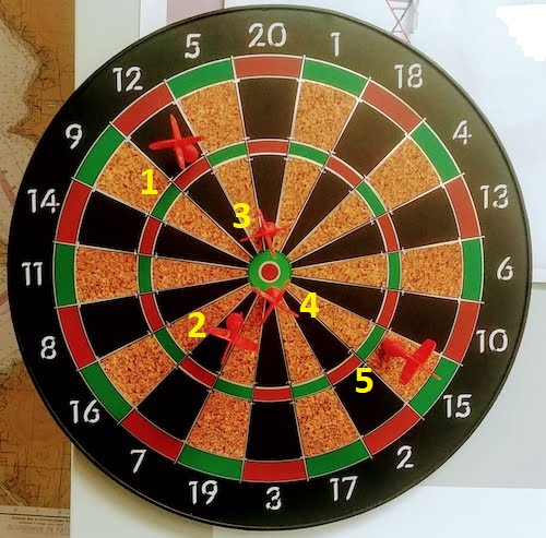
Figure 1. Magnetic dart board with 5 darts. Click image to view full sized image.
The distance in centimeters (cm) between where each of the five darts landed on the board compared to the bullseye is reported in (Table 1),
Table 1. Results of five darts thrown at a target (Figure 2)*
| Dart | Distance |
|---|---|
| 1 | 7.5 |
| 2 | 3.0 |
| 3 | 1.0 |
| 4 | 2.7 |
| 5 | 7.4 |
* distance in centimeters from the center.
Note 1: Use of the coordinate plane, and including the angle measurement in addition to distance (the vector) from center, would be a better analysis. In the context of darts, determining accuracy of a thrower is an Aim-Point targeting problem and part of your calculation would be to get MOA (minute of angle). For the record, the angles (degrees) were
| Dart | Distance | Angle |
|---|---|---|
| 1 | 7.5 | 124.4 |
| 2 | 3.0 | -123.7 |
| 3 | 1.0 | 96.3 |
| 4 | 2.7 | -84.3 |
| 5 | 7.4 | -31.5 |
measured using imageJ. Because there seems to be an R package for just about every data analysis scenario, unsurprisingly, there’s an R package called shotGroups to analyze shooting data.
How precise was the dart thrower? We’ll use the coefficient of variation as a measure of precision. Second, how accurate were the throws? Use R to calculate
darts = c(7.5, 3.0, 1.0, 2.7, 7.4)
#use the coefficient of variation to describe precision of the throws
coefVar = 100*(sd(darts)/mean(darts)); coefVar
[1] 68.46141
Confidence Interval to describe accuracy.
For a game of darts, the true value would be a distance of zero — all bullseyes. We need to calculate the standard error of the mean (SEM), then, we calculate the confidence interval around the sample mean.
#Calculate the SEM
SEM <- sd(darts)/sqrt(length(darts)); SEM
[1] 1.322649
#now, get the lower and upper limit, subtract from the mean
confidence <- c(mean(darts)-2*SEM, mean(darts), mean(darts)+2*SEM); confidence
[1] 1.674702, 4.320000, 6.965298
The mean was 4.3 cm, therefore to get the lower limit of the interval subtract 2.65 (2*SEM = 2.645298) from the mean; for the upper limit add 2.65 to the mean. Thus, we report our approximate confidence interval as (1.7, 7.0), and we read this as saying we are about 95% confident the population value is between these two limits. Five is a very small sample number, so we shouldn’t be surprised to learn that our approximate confidence interval would be less than adequate. In statistical terms, we would use the t-distribution, and not the normal distribution, to make our confidence interval in cases like this.
Note 2: As a rule, implied by Central Limit theory and use of asymptotic statistical estimation, a sample size of 30 or more is safer, but probably unrealistic for many experiments. This is sometimes called as the rule of thirty. (For example, a 96-well PCR array costs about $500; with n = 30, that’s $15,000 US Dollars for one group!). So, what about this rule? This type of thinking should be avoided as “a relic of the pre-computer era,” (Hesterberg, T. (2008). It’s Time To Retire the” n>= 30″ rule.). We can improve on asymptotic statistics by applying bootstrap principles (Chapter 19).
We made a quick calculation of the confidence interval; we can get make this calculation by hand by incorporating the t distribution. We need to know the degrees of freedom, which in this case is 4 (n – 1, where n = 5). We look up critical value of t at 5% (to get our 95% confidence interval), t = 2.78. Subtract for lower limit t*SEM and add for upper limit t*SEM to the sample mean for the 95% confidence interval.
We can get help from R, by using the one-sample t-test with a test against the hypothesis that the true mean is equal to zero. Among a variety of output we will introduce later (see Chapter 8 and 10), the confidence interval is reported (yellow highlight),
#make an attach a data frame object
Ddarts <- data.frame(darts)
t.test(darts,mu=0)
One Sample t-test
data: darts
t = 3.2662, df = 4, p-value = 0.0309
alternative hypothesis: true mean is not equal to 0
95 percent confidence interval:
 0.6477381 7.9922619
sample estimates:
mean of x
 4.32
t.test uses the function qt(), which provides the quantile function. To recreate the 95% CI without the additional baggage output from the t.test, we would simply write
#upper limit
mean(darts)+ qt(0.975,df=4)*sd(darts)/sqrt(5)

#lower limit
mean(darts)+ qt(0.025, df = 4, lower.tail=TRUE)*sd(darts)/sqrt(5)
where sd(darts)/sqrt(5) is the standard error of the mean.
Or, alternatively, download and take advantage of a small package called Rmisc (not to be confused with the RcmdrMisc package) and use the function CI
library(Rmisc)
CI(darts)
     upper     mean     lower
7.9922619 4.3200000 0.6477381
The advantage of using the CI() command from the package Rmisc is pretty clear; I don’t have to specify the degrees of freedom or the standard error of the mean. By default, CI reports the 95% confidence interval. we can specify any interval simply by adding to the command. For example,
CI(darts, ci=0.90)
reports upper and lower limits for the 90% confidence interval.
Try it. On your own, get the 90% confidence interval and the 99% confidence intervals for our dart example. Compare to the 95% confidence interval — what do you conclude about “confidence” in our estimate from 90% to 99%?
Confidence intervals from p-values.
And finally, it is not unusual for a report to provide summary statistics, differences between means (ie, effect size), and p-values (orange highlight), but not report confidence intervals. We discuss p-values and the concept of statistical significance beginning in Chapter 8. But for now, we show how to calculate approximate confidence intervals from the p-value. This may be of use for conducting meta-analysis (Chapter 20.15). See two helpful “how to” articles by Bland and Altman in 2011 BMJ (references listed in Chapter 3.6 – References).
In brief, calculate the test statistic for a normal distribution (letZ), calculate a standard error, and then the lower and upper limits for the 95% confidence interval. We illustrate use of the calculator formulas with the dart example, the p-value was 0.0309; the estimate was 4.32.
R code
letZ = (-0.862 + sqrt(0.743 - 2.404*log(0.0309, base = exp(1)))) = 2.154903
letSE = 4.32/letZ = 2.00473
1.96*letSE = 3.929271 # Add for upper and subtract for lower
The lower limit is 0.39 (4.32 – 3.929271) and the upper limit is 8.25 (4.32 + 3.929271). Although in the ballpark, these calculated estimates are wider than the confidence interval estimated by the t.test command. Small sample size, n = 5, is to blame — the accuracy of these methods, based on asymptotic statistical estimation approaches, assumes the law of large numbers applies.
Significant figures.
And finally, we should respect significant figures, the number of digits which have meaning. Our data were measured to the nearest tenth of a centimeter, or two significant figures. Therefore, if we report the confidence interval as (0.6477381, 7.9922619), then we imply a false level of precision, unless we also report our random sampling error of measurement.
R has a number of ways to manage output. One option would be to set number of figures globally with the options() function — all values reported by R would hold for the entire session. For example, options(digits=3) would report all numbers to three significant figures. Instead, I prefer to use signif() function, which allows us to report just the values we wish and does not change reporting behavior for the entire session.
signif(CI(darts),2)
upper  mean lower
 8.00  4.30  0.65
Note 3: The options() function allows the R user to set a number of settings for an R session. After gaining familiarity with R, the advanced user recognizes that many settings can be changed to make the session work to report in ways more convenient to the user. If curious, submit options() at the R prompt and available settings will be displayed.
The R function signif() applies rounding rules. We apply rounding rules when required to report estimates to appropriate levels of precision. Rounding procedures are used to replace a number with a simplified approximation. Wikipedia provides a comprehensive list of rounding rules. Notable rules include
- directed rounding to an integer, eg, rounding up or down
- rounding to nearest integer, eg, round half up (down) if the number ends with 5
- randomly rounding to an integer, eg, stochastic rounding.
With the exception of stochastic rounding, all rounding methods impose biases on the sets of numbers. For example, the round half up method applied for numbers above 5, round down for numbers below 5 will increase the variance of the sample. In R, use round() for most of your work. If you need one of the other approaches, for example, to round up, the command is ceiling(); to round down we use floor().
When to round?
No doubt your previous math classes have cautioned you about the problems of rounding error and their influence on calculation. So, as a reminder, if reporting calls for rounding, then always round after you’ve completed your calculations, never during the calculations themselves.
A final note about significant figures and rounding. While the recommendations about reporting statistics are easy to come by (and often very proscriptive, eg, Table 1, Cole 2015), there are other concerns. Meta-analysis, which are done by collecting information from multiple studies, would benefit if more and not fewer numbers are reported, for the very same reason that we don’t round during calculations.
Questions
- Calculate the correct 90% and 99% confidence intervals for the dart data using the t-distribution
- by hand
- by one alternative method in R, demonstrated with examples in this page
- How many significant figures should be used for the volumetric pipettor p1000? The p200? The p20 (data at end of this page)?
- Another function,
round(), can be used. Try
round(CI(darts),2)
-
- and report the results: vary the significant figures from 1 to 10 (
signif()will take digits up to 22). - See any output differences between
signif()andround()? Don’t forget to take advantage of R help pages (eg, enter?roundat the R prompt) and see Wikipedia.
- and report the results: vary the significant figures from 1 to 10 (
- Compare rounding by
signif()andround()for the number 0.12345. Can you tell which rounding method the two functions use? - Calculate the coefficient of variation (CV) for each of the three volumetric pipettors from the data at end of this page. Rank the CV from smallest to largest. Which pipettor had the smallest CV and would therefore be judged the most precise?
- (data provided at end of this page, click here).
- Standards distinguish between within run precision and between run precision of a measurement instrument (see Chapter 16.5 – Instrument reliability and validity). The data in Table 1 were all recorded within 15 minutes by one operator. What kind pf precision was measured?
- Calculate the standard error of the means for each of the three pipettors from the data
- (data provided at end of this page, click here).
- Calculate the approximate confidence interval using the 2SE rule and judge which of the three pipettors is the most accurate (narrowest confidence interval)
- Repeat, but this time apply your preferred R method for obtaining confidence intervals.
- Compare approximate and R method confidence intervals. How well did the approximate method work?
- Return to the dart example, but now assume the p-value was p = 0.003 and again for p = 0.0003. Estimate the 95% confidence interval for each case; the difference remains 4.32. How does the change in p-value, from 0.03 to 0.0003 — a two orders of magnitude difference — affect the estimates for the confidence interval (hint: describe the width of the CI)?
Quiz Chapter 3.5
Statistics of error
Data sets
Pipette calibration
| p1000 | p200 | p100 |
|---|---|---|
| 0.113 | 0.1 | 0.101 |
| 0.114 | 0.1 | 0.1 |
| 0.113 | 0.1 | 0.1 |
| 0.115 | 0.099 | 0.101 |
| 0.113 | 0.1 | 0.101 |
| 0.112 | 0.1 | 0.1 |
| 0.113 | 0.1 | 0.1 |
| 0.111 | 0.1 | 0.1 |
| 0.114 | 0.101 | 0.101 |
| 0.112 | 0.1 | 0.1 |
Chapter 3 continues
3.4 – Estimating parameters
Introduction.
What you will find on this page. Definitions for constants, variables, and parameters as used in data analytics. Statistical bias and the concept of unbiased estimators are discussed. The different types of error are introduced along with definitions of accuracy and precision. Statistics used to quantify error are presented in the next section, Chapter 3.4.
Estimating parameters.
Parameters belong to populations; they are fixed but unknown. Parameters are characteristics of populations: the typical average height and weight of five year old children; What is the normal range of values for height and weight of five year old children; average and range of gene expression of TP53 in epithelial lung cells of 50 year old non-smoking humans; etc. Because we generally do not have at our disposal surveys — census — of entire populations for these characteristics, we sample and calculate descriptive statistics for a subset of individuals from populations: these statistics, the mean height, range of height, etc., are variables. We expect average height, range of height, etc., to change, to vary, from sample to sample. A constant, as the word implies, is not variable and remains unchanged.
We estimate parameters (means, variances) from samples of observations from a population. Intuitively then, our estimates are only as good as how representative of the population the sample is. Statistics allows us to be more precise: we can define “how good” our estimates are by asking about, and quantifying, the accuracy and precision of our estimates.
Notwithstanding the notion of “personalized medicine,” our goal in science is to understand cause and effect among sets of observations on samples from a population. We ask, what is the link between lung cancer and smoking? We know that smoking tobacco cigarettes increases risk of cancer, but not everyone who smokes will get cancer (Pesch et al., 2012). Tumorigenic risk is in part mediated by heredity (cf. Trifiletti et al 2017). That’s one way we run into problems in statistics: the biological phenomenon is complicated in ways we are not yet aware of, and thus samples drawn from populations are heterogeneous. Put another way, we think there is one population, but there may be many distinct populations. By chance, repeated samples drawn from the population include individuals with different risk associated with heredity.
As an aside, this is precisely why the concept of personalized medicine is important. Medical researchers have learned that some people with breast cancer respond to treatment with trastuzumab, a monoclonal antibody, but others do not (review in Valabrega et al 2007). Responders have more copies of a gene, copy number variation, for an EGF-like receptor called HER2. In contrast, non-responders to trastuzumab have fewer copies of this receptor (and are said to be HER2-negative in an antibody test for HER2). Thus, we speak about people with breast cancer as if the disease is the same, and from a statistical point of view, we would assume that individuals with breast cancer are of the same population. But they are not — and so the treatment fails for some, but works for others. In this example, we have a mechanism or cause to explain why some do not respond; their breast cancer is not associated with increased copy numbers of HER2. And so in studies with breast cancer, statisticians may account for differences in HER2 status. Note: Fewer than 30% of breast cancer may have over-expression of HER2, (Bilous et al. 2003).
Clearly, HER2 status would be used by statisticians when drawing samples from population, and we would not mistake samples. But, in many other situations we are not aware of any differences and so we assume our samples come from the same population. Note that even with imperfect knowledge about samples, experimental design is intended to help mediate heterogeneous samples. For example, this is why treatment controls need to be used, or case controls are included in studies.
Random assignment to groups also is an attempt to control for unknowns: if random, then all treatment groups will likely include representatives of the numerous co-factors that contribute to risk.
Statisticians have an additional, technical burden: there are often a variety of ways (algorithms) to describe or make inferences about samples, and they are not equally capable of giving us “truth.” Estimates of a parameter are not going to be exactly the true value of the parameter! This is the problem of identifying unbiased ways to estimate parameters. In statistics, bias quantifies whether an algorithm to calculate a particular statistic (e.g., the mean or variance), is consistently too low or too high.
Random sampling.
Random sampling from the population is likely to be our best procedure for obtaining representative samples, but it is not foolproof (we’ll return to situations where random sampling fails to provide adequate samples of populations in Chapter 5.5 Importance of randomization in experimental design). However, a second concern is how to calculate the mean, how to calculate the variance. In the section on Descriptive Statistics (Chapter 3.2), we presented how to calculate the arithmetic mean — the simple average — but also introduced you to other calculations for the middle (e.g., median, geometric mean, harmonic mean). How to know which “middle” is correct?
Statisticians use the concept of bias — the simple arithmetic mean is an unbiased estimator of the population parameter, but a correction needs to be made to the calculation of sample variance to remove bias. Bias implies that the estimator systematically misses the target in some way. Good or “best” parameter estimates are, on average, going to be close to the actual parameter if we collected many samples of the population (this will depend on the sample size and the variability of the data). Earlier we introduced Bessel’s correction to the sample variance, divide the sum of squares by n – 1 and not N as we did for the population variance, so that it is an unbiased estimator of the sample variance. Thus, statisticians have worked out how well their statistical equations work as estimators; concepts of expected values or the expectation are used to evaluate how well an estimator works. In statistics, the expected value of a statistic is calculated by multiplying each of the possible outcomes by the likelihood each outcome will occur and then summing all of those values..
We need to add a bit more to our discussion about measurement and estimation.
Types of error.
To measure is to assign a number to something, a variable. Measurements can have multiple levels, but are of the four data types: nominal, ordinal, interval scale, and ratio scale. Nominal and ordinal types are categorical or qualitative; interval and ratio are continuous or quantitative. Errors in measurement represent differences between what is observed and recorded compared with the true value, i.e., the actual population value. With respect to measurement we distinguish between random errors and systematic errors. Random errors occur by chance, and are thus expected to vary from one measurement instance from another. Random error may lead to measures larger or smaller than the true value. Systematic errors are of a kind that can be attributed to failures of an experimental design or instrument.
Accuracy is reflected in the question: how close to the true value is our measure? Accuracy is distinct from precision, the concept of how clustered together are repeated values for the same measurement. All measurement has associated error, which may be divided into two kinds: random error and systematic error.
We tend to think of error in terms of mistakes, mistakes by us or as failure of the measurement process. However, in biology research, that is too restrictive of a meaning for error. First, experimental error occurs when the estimates derived from the samples — sample mean, sample variance — differ from the population parameters — population mean, population variance. Second, error in biology ranges from mistakes in data collection to real differences among individuals for a characteristic. The latter source, error among individuals, is of course, not a mistake, but rather, it’s the “very spice of life” (Cowper 1845). We’ll leave the study of individual differences, biological error, for later. This section is concerned with error in the sense of mistakes.
Random error includes things like chance error in an instrument leading to different repeat measures of the same thing and to the reality that individual differences exist for most biological traits. We minimize the effects of this kind of error by randomizing: we randomly select samples from populations; we randomly assign samples to treatment groups. Random error can make it hard to differentiate treatment effects. Random error decreases precision, the repeatability of measures. At worse, random error is conservative — it tends to mean we miss group differences, we conclude that the treatment (e.g., aspirin analgesics) has no effect on the condition (e.g., migraines). This kind of error is referred to as a Type II error (Chapter 8).
The experimental design remedy for random error is to increase sample size, a key conclusion drawn from power analysis on experiments, discussed in Chapter 11. The other type of error, systematic error, a type of bias, is more in line with the idea of errors being synonymous with mistakes. Uncalibrated instruments yield incorrect measures. And these kinds of errors lead us to make errors that can be more problematic. An example? Back in the early 1990s when I started research on whole animal metabolic rates (e.g., Dohm et al 1994, Beck et al 1995), we routinely set baseline carbon dioxide, CO2, levels to 0.035% of volume of dry air (350 ppm, parts per million), which reflected ambient levels of CO2 at the time (see Figure 4 in Chapter 4.6).
#NOAA monthly data from Mauna Loa Observatory
co2.1994 <- c(358.22, 358.98, 359.91, 361.32, 361.68, 360.80, 359.39, 357.42, 355.63, 356.09, 357.56, 358.87)
You are probably aware, today, background CO2 have increased considerably even since the 1980s. Data for 2021 (average 420 ppm — reporting just 2 significant figures) are provided below
co2.2021 <- c(415.49, 416.72, 417.61, 419.01, 419.09, 418.93, 416.9, 414.42, 413.26, 413.9, 414.97, 416.67)
source: Global Monitoring Lab, NOAA
Thus, if I naively compared rates of CO2 produced by an animal at rest,  , measured today against the data I gathered back in the 1990s without account for the change in background CO2 in my analysis, I will have committed a systematic error: values of on animals would be systematically higher than values for 1988 when I apply a baseline correction.
Examples of error.
One under-reported cost of next-generation sequencing technologies is that base calls, the process of assigning a nucleotide base to chromatogram peaks has more errors than traditional Sanger-based sequencing methods (Fox et al 2014). In “next-generation-sequencing” (NGS) methods, individual DNA fragments are assigned sequences, whereas Sanger methods took the average sequence of a collection of DNA fragments; thus, in principle, NGS methods should be able to characterize variation of mixtures of sequences in ways not available to traditional sequencing approaches. However, artifacts introduced in sample preparation and PCR amplification lead to base calling errors (Fox et al 2014).
Gene expression levels will differ among tissue types, thus mixed samples from different tissues will misrepresent gene expression levels.
Measurement of energy expenditure, oxygen uptake and carbon dioxide release by an organism, have long been sources of study in ecology and other disciplines. A classic measure is called basal metabolic rate, measured as the rate of oxygen consumption of an endothermic animal, post-absorptive (i.e., not digesting food), at rest but not sleeping, while the animal is contained within a thermal-neutral environment (Blaxter 1989).
Accuracy and precision.
Two properties of measurement are the accuracy of the measure and its precision. Accuracy is defined as the closeness of a measured value to its true value. Precision refers to the closeness of a second measure to the first, to the closeness of a third measure to the first and second, and so on. Precision refers to repeatability of measurement. We suggested use of the coefficient of variation, defined with examples in Chapter 3.2, as a way to quantify precision.
Consider the accuracy and precision of three volumetric pipettors: p1000, which has a nominal range between 100 and 1000 μL (microliters); p200, which has a range between 20 and 200 μL; p100, which has a range between 10 and 100 μL. Which of these three pipettors do you think would have the best accuracy and precision for dispensing 100 μL? We can test pipettors by measuring the mass of distilled water dispensed by the pipettor on an analytical balance. For 100 μL of distilled water at standard temperature and pressure conditions, the mass of the water would be 0.100 grams. The results are shown in the table, and a dot plot is shown in the figure to help us see the numbers.
Table 1. Mass (grams) of 100 μL of distilled water dispensed by three volumetric pipettors*
| p1000 | p200 | p100 | |
| 0.113 | 0.100 | 0.101 | |
| 0.114 | 0.100 | 0.100 | |
| 0.113 | 0.100 | 0.100 | |
| 0.115 | 0.099 | 0.101 | |
| 0.113 | 0.100 | 0.101 | |
| 0.112 | 0.100 | 0.100 | |
| 0.113 | 0.100 | 0.100 | |
| 0.111 | 0.100 | 0.100 | |
| 0.114 | 0.101 | 0.101 | |
| 0.112 | 0.100 | 0.100 | |
| mean: | 0.113 | 0.100 | 0.1004 |
| standard deviation: | 0.0012 | 0.0005 | 0.0005 |
*Temperature 21.5 °C, barometric pressure 76.28 cm mercury (elevation 52 meters). Data presented in Table 1 were not corrected to standard temperature or pressure.
Here is the code for the R run; assuming that you have started R commander, then copy and paste each line into the R Commander script window; if not, enter the script one line at a time in the R console. Recall that the hashtag, #, is used to add comment lines.
Note 1: A reminder: Don’t include the last two rows from Table 1 in your data set; these contain descriptive statistics and are not your data.
#create the variables
p1000 <- c(0.113, 0.114, 0.113, 0.115, 0.113, 0.112, 0.113, 0.111, 0.114, 0.112)
p100 <- c(0.101, 0.1, 0.1, 0.101, 0.101, 0.1, 0.1, 0.1, 0.101, 0.1)
p200 <- c(0.1, 0.1, 0.1, 0.099, 0.1, 0.1, 0.1, 0.1, 0.101, 0.1)
#create a data frame
pipet <- data.frame(p100,p200,p1000)
attach(pipet)
#stack the data
stackPipet <- stack(pipet[, c("p100","p200","p1000")])
#Add variable names
names(stackPipet) <- c("mass", "pipet")
#create the dot plot
with(stackPipet, RcmdrMisc::Dotplot(mass, by=pipet, bin=FALSE))
From Table 1 we see that the means for the p100 and p200 were both close to the target mass of 0.1 g. The mean for the p1000, however, was higher than the target mass of 0.1 g. A dot plot is a good way to display measurements (Fig. 1).
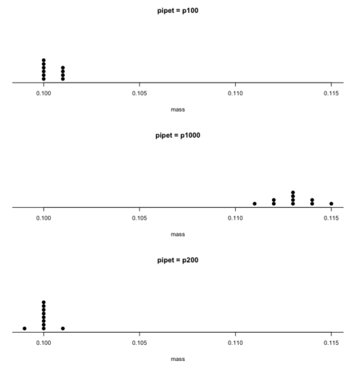
Figure 1. Dot plot of pipet results.
Note 2: Dotplot() is part of the RcmdrMisc package; if you are using the Rcmdr script window (please do!), then the functions in RcmdrMisc are already available and you wouldn’t need to use RcmdrMisc:: (package name plus double-colon operator) to call the Dotplot() function (more properly, referred to as namespaces). Thus, with(stackPipet, Dotplot(mass, by=pipet, bin=FALSE)) would work perfectly well within the Rcmdr script window.
From the dot plot we can quickly see that the p1000 was both inaccurate (the data fall well above the true value), and lacked precision (the values were spread about the mean value). The other two pipettors showed accuracy and looked to be similar in precision, although only two of ten values for the p200 were off target compared to four of ten values for the p100. Thus, we would conclude that the p200 was best at dispensing 100 microliters of water.
In the next chapter we apply statistics to estimate our confidence in this conclusion. In contrast to measurement, estimation implies calculation of a value. In statistics, estimates may be a point, e.g., a value of a collection of data, or an interval, e.g., a confidence interval.
Summary.
This is your first introduction into the concept of experimental design, as defined by statisticians! One of the key tasks for a statistical analyst is to have an appreciation for measurement accuracy and precision as established in the experiment. Precise and accurate measurement levels determine how well questions about the experiment can be answered. At one extreme, if a measure is imprecise, but accurate, then it will be challenging to quantify differences between a control group and a treatment group. At the other extreme, if the measure is precise, but inaccurate, the danger would be differences between the treatment and control group may be more likely, even when the groups are truly not different!
Questions.
- List the types of error in measuring mRNA expression levels on a gene for a sampling of cells from biopsy of normal tissue and a biopsy of a tumor. Assume use of NEXGEN methods for measuring gene expression. Distinguish between technical errors and biological errors.
- If confidence interval are useful for estimating accuracy, what statistic do we call to quantify precision?
Quiz Chapter 3.4
Estimating parameters
Chapter 3 contents
8.3 – Sampling distribution and hypothesis testing
Introduction
Understanding the relationship between sampling distributions, probability distributions, and hypothesis testing is the crucial concept in the NHST — Null Hypothesis Significance Testing — approach to inferential statistics. is crucial, and many introductory text books are excellent here. I will add some here to their discussion, perhaps with a different approach, but the important points to take from the lecture and text are as follows.
Our motivation in conducting research often culminates in the ability (or inability) to make claims like:
- “Total cholesterol greater than 185 mg/dl increases risk of coronary artery disease.”
- “Average height of US men aged 20 is 70 inches (1.78 m).”
- “Species of amphibians are disappearing at unprecedented rates.”
Lurking beneath these statements of “fact” for populations (just what IS the population for #1, for #2, and for #3?) is the understanding that not ALL members of the population were recorded.
How do we go from our sample to the population we are interested in? Put another way — How good is our sample? We’ve talked about how “biostatistics” can be generalized as sets of procedures you use to make inferences about what’s happening in populations. These procedures include:
- Have an interesting question
- Experimental design (Observational study? Experimental study?)
- Sampling from populations (Random? Haphazard?)
- Hypotheses: HO and HA
- Estimate parameters (characterize the population)
- Tests of hypotheses (inferences)
We have control of each of these — we choose what to study, we design experiments to test our hypotheses…We have already introduced these topics (Chapters 6 – 8).
We also obtain estimates of parameters, and inferential statistics applies to how we report our descriptive statistics (Chapter 3). Estimates of parameters like the sample mean and sample standard deviation can be assessed for accuracy and precision (eg, confidence intervals).
Sampling distribution
Imagine drawing a sample of 30 from a population, calculating the sample mean for a variable (eg, systolic blood pressure), then calculating a second sample mean after drawing a new sample of 30 from the same population. Repeat, accumulating one estimate of the mean, over and over again. What will be the shape of this distribution of sample means? The Central Limit Theorem states that the shape will be a normal distribution, regardless of whether or not the population distribution was normal, as long as the sample size is large (ie, Law of Large Numbers). We alluded to this concept when we introduced discrete and continuous distributions (Chapter 6).
It’s this result from theoretical statistics that allows us to calculate the probability of an event from a sample without actually carrying out repeated sampling or measuring the entire population.
A worked example
To demonstrate the CLT we want R to help us generate many samples from a particular distribution and calculate the same statistic on each sample. We could make a for loop, but the replicate() function provides a simpler framework. We’ll sample from the chi-square distribution. You should extend this example to other distributions on your own, see Question 5 below.
Note 1: This example is much simpler to enter and run code in the script window, modifying code directly as needed. If you wish to try to run this through Rcmdr, you’ll need to take a number of steps, and likely need to modify the code and rerun anyway. Some of the steps in would be Rcmdr: Distributions → Continuous distributions → Chi-squared distribution → Sample from chi-square distribution…, then running Numerical summaries and saving the output to an object (eg, out), extracting the values from the object (eg, out$Table, confirm by running command str(out)— str() is an R utility to display the structure of an object), then testing the object for normality Rcmdr: Statistics → Test of normality, select Shapiro-Wilk, etc.. In other words, sometimes a GUI is a good idea, but in many cases, work with the script!
Generate x replicate samples (eg, x = 10, 100, 1000, one million) of 30 each from chi-square distribution with one degree of freedom, test the distribution against null hypothesis (assume normal distributed, eg, Shapiro-Wilk test, see Chapter 13.3), then make a histogram (Chapter 4.2), like Figure 1 or Figure 2.
x.10 <- replicate(10, {
my.mean <- rchisq(30, 1)
mean(my.mean)
})

normalityTest(~x.10, test="shapiro.test")
hist(x.10, col="orange")
Result from R
Shapiro-Wilk normality test

data: x.10
W = 0.87016, p-value = 0.1004
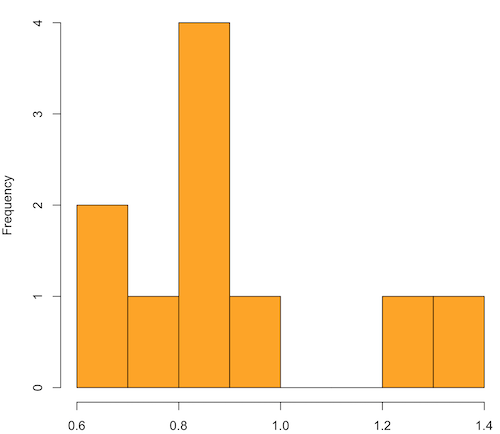
Figure 1. means of ten replicate samples drawn at random from chi-square distribution, df = 1.
Modify the code to draw 100 samples, we get Fig 2.
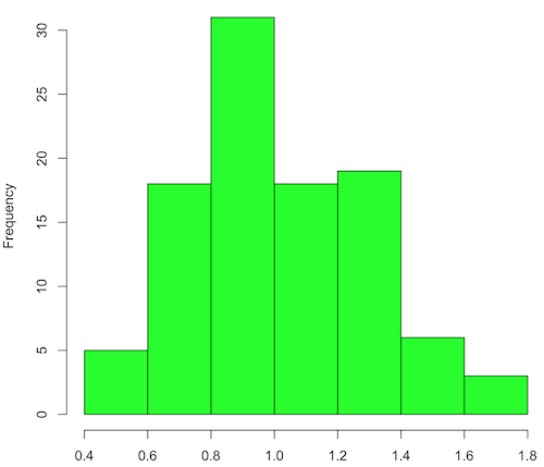
Figure 2. means of 100 replicate samples drawn at random from chi-square distribution, df = 1. Results from Shapiro-Wilks test: W = 0.97426, p-value = 0.04721.
And finally, modify the code to draw one million samples, we get Figure 3.
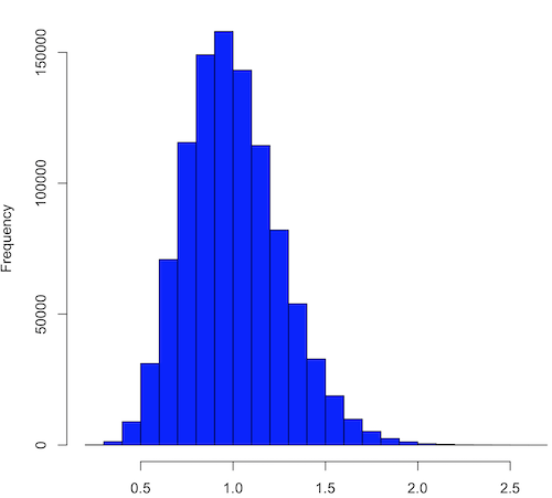
Figure 3. means of one million replicate samples drawn at random from chi-square distribution, df = 1. Normality test will fail to run, sample size of 5000 limit.
How to apply sampling distribution to hypothesis testing
First, a reminder of some definitions.
Estimate = we will always (almost) concern ourselves with how good our sample mean (such values are called estimates) is relative to the population mean, the thing we really want, but can only hope to get an estimate of.
Accuracy = how close to the true value is our measure?
Precision = how repeatable is our measure?
How can we tell if we have a good estimate? We want an estimate with an evaluation for accuracy and for precision. The sampling error provides an assessment of precision, whereas the confidence interval provides a statement of accuracy. We need an estimate of the sampling error for the statistic,
Sample standard error of the mean
We introduced sample error of the mean in section 3.4 of Chapter 3. Everything we measure can have a corresponding statement about how accurate (sampling error) is our estimate! First, we begin by asking, “how accurate is the mean that we estimate from a sample of a population?” How do we answer this? We could prove it in the mathematical sense of proof (and people have and do) OR we can use the computer to help. We’ll try this approach in a minute.
What we will show relates to the standard error of the population mean (SEM) or

, whose equation is shown below.

or equivalently, from the standard deviation we have
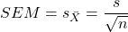
Note that the SEM takes the variance and divides through by the sample size. In general, then, the larger the sample size, the smaller the “error” around the mean. As we work through the different statistical tests, t-tests, analysis of variance, and related, you will notice that the test statistic is calculated as a ratio between a difference or comparison divided by some form of an error measurement. This is to remind you that “everything is variable.”
A note on standard deviation (SD) and standard error of the mean (SEM): SD estimates the variability of a sample of Xi‘s whereas SEM estimates the variability of a sample of means.
Let’s return to our thought problem and see how to demonstrate a solution. First, what is the population? Second, can we get the true population mean?
One way, a direct (but impossible?) approach would be to measure it — get all of the individuals in a population and measure them, then calculate the population mean. Then, we could compare our original sample mean against the true mean and see how close it was. This can be accomplished in some limited cases. For example, the USA conducts a census of her population every ten years, a procedure which costs billions of dollars. We can then compare samples from the different states or counties to the USA mean. And these statistics are indeed available via the census.gov website. But even the census uses sampling — individuals are randomly selected to answer more questions and from this sample trends in the population are inferred.
So, sampling from populations is the way to go for most questions we will encounter. The procedures we will use to show how a sample mean relates to the population mean are general and may be used to show how any estimate of a variable (sample mean and sample standard deviation, etc.), relates to properties of a parameter. We’ll get to the other issues, but for now, think about sample size.
Sampling from populations is necessary and inevitable, and, to a certain extent, under your control. But how many individuals do we need? The quick answer is for me to direct your attention to the equation for the SEM. Can you see in that ratio the secret to obtaining more precise estimates? There are many ways to approach this question, but let’s use the tools from last time, those based on properties of a normal distribution.
If we can view the sampling as having come from a population at least approximately normally distributed for our variable, then we can now examine empirically the effect of different sample sizes on the estimate of the mean.
A hint: variability is important!
From one population we obtain two samples, A and B. Sample sizes are
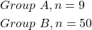
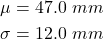
Assume for now that we know the true mean (μ) and standard deviation (σ) for the population. Note. This is one of the points of why we use computer simulation so much to teach statistics — it allows us to specify what the truth is, then see how our statistical tools work or how our assumptions affect our statistically based conclusions.
Confidence intervals
Reliability is another word for precision. We define a confidence interval as a statistic to report the reliability of our estimated statistic. We introduced confidence interval in Chapter 3.4. At least in principle, confidence intervals can be calculated for all statistics (mean, variance, etc.,) and for all data types. Confidence intervals define a lower limit, L, and an upper limit, U, and that you are making a statement that you are “95% certain that the true value (parameter value) is between these two limits.
We previously reported how to calculate an approximate confidence intervals for proportions and for NNT; simply multiple standard error estimate by 2. Here we introduce an improved approximate calculation of the 95% confidence interval for the sample mean

where Z is something you would look up from the table of the normal distribution. For a 95% confidence interval, 100% – 95% = 5% and divide 5% by two: the lower limit corresponds to 2.5% and the upper limit corresponds to 2.5% on our normal distribution. We look up the table and we find that Z for 0.025 is 1.96 and that is the value we would plug into our equation above. For large sample sizes, you can get a pretty decent estimate of the confidence interval by replacing 1.96 with “2.”
Questions
1. What is the probability of having a sample mean greater than 50 (mean > 50) for a sample of n = 9 ?
We’ll use a slight modification of the Z-score equation we introduced in Chapter 6.6 — the modification here is that previously we referred to the distribution of Xi‘s and how likely a particular observation would be. Instead, we can use the Z score with the standard normal distribution (aka Z-distribution), approach to solving how likely an estimated sample mean is given the population parameters μ and σ. Recall the Z score

We have everything we need except the SEM, which we can calculate by dividing the standard deviation by squared root of sample size.
For

, σ = 12.0 (given above), and μ = 47, n = 9, plug in the values:
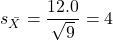
Therefore, after applying the equation for Z score,  . This corresponds to how far away from the standard mean of zero.
Look up from the table of normal distribution. The answer is  , which corresponds to that
 is EQUAL to or GREATER than 0.75, which is what we wanted. Translated, this implies that, given the level of variability in the sample, 22.66% of your sample means would be greater than 50! We write:
 .
Some care needs to be taken when reading these tables — make sure you understand how the direction (less than, greater than) away from the mean is tabulated.
2. Instead of greater, how would you get the probability less than 50?
Total area under the curve is 1 (100%), so subtract  .
I recommend that you do these by hand first, then check your answers. You’ll need to be able to do this for exams.
Here’s how to use Rcmdr to do these kind of problems.
Rcmdr: Distributions → Continuous distributions → Normal distribution → Normal probabilities …
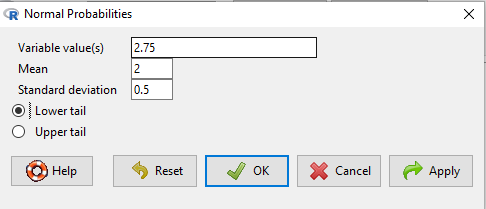
Figure 5. Screenshot Rcmdr menu to get normal probability.
Here’s the answer from Rcmdr
pnorm(c(50), mean=47, sd=12, lower.tail=TRUE)

[1] 0.5987063
3. Now, try a larger sample size. For  , what is the probability of having a sample mean greater than 50 (
 )?
, μ = 47, σ = 12, n = 50 and

Therefore, after applying the equation for Z score,  . Look up (Normal table, subtract answer from 1) and we get
 .
Or 3.84% of your sample means would be greater than 50! We write:  .
Said another way: If you have a sample size of 50 () and you obtain a mean greater than 50 then there is only a 3.84% chance that the TRUE MEAN IS 47.
4. What happens if the variability is smaller? Chance σ from 12 to 6 then repeat questions 1 and 4.
5. Repeat the demonstration of Central Limit Theorem and Law of Large Numbers for discrete distributions
- binomial distribution. Replace
rchisq()withrbinom(n, size, prob)in thereplicate()function example. See Chapter 6.5 - poisson distribution. Replace
rchisq()withrpois(n, lambda)in thereplicate()function example. See Chapter 6.5
Quiz Chapter 8.3
Sampling distribution and hypothesis testing
Chapter 8 contents
- Introduction
- The null and alternative hypotheses
- The controversy over proper hypothesis testing
- Sampling distribution and hypothesis testing
- Tails of a test
- One sample t-test
- Confidence limits for the estimate of population mean
- References and suggested readings
5.3 – Replication, Bias, and Nuisance Variables
Introduction
This page describes additional elements of experimental design, replication and bias, which can impact the validity of a study.
Replication in science refers to repeating an experiment under identical conditions multiple times. To the extent the same conclusions are achieved, we can say the outcome is reproducible (Simmons 2014) and, therefore, likely to be objectively true (Earp 2011). Replication of experimental and sampling units is an essential component of good experimental design. Confusing technical replicates for biological replicates is called pseudoreplication.
Bias refers to any of a number of sociological and cognitive errors which may influence conclusions in science (Ionnidis 2005). In a meta-analysis, Fanelli et al (2017) reported that while the size of effect from identifiable biases were small, some disciplines were more prone to these sources of error. That researchers testing similar hypotheses reach different conclusions may result from bias. One such bias is positive outcome bias, where reports of null hypotheses are more often rejected than they should be based on sample size and other concerns of statistical power (see Chapter 11 – Power analysis).
The page concludes with a discussion of nuisance variables, variables that may be causally associated with the outcome of interest, but themselves are either of no interest in the study, or may not be known in advance (Meehl 1970; see also discussion of spurious correlations in Chapter 16.3 – Data aggregation and correlation).
Technical vs. biological replicates.
A laboratory technician retrieves a vial of an immortalized cell line from cryostorage and initiate propagation of the cells for the week’s work. After a couple of days of subculturing, the technician has grown millions of cells and is ready to set up an assay. After washing the cells in PBS (phosphate buffered saline), the technician adjusts the concentration of cells to 10,000 per mL media, places the tube on ice, and proceeds to set up a 48 well microplate. To each well, the technician adds media, one or more agents (Table 1), plus cells, total volume each well at one mL, three replicates per treatment.
Table 1. In our example there were four treatments plus a control (media only)
- DMSO only (D)
- DMSO + Cytokine (DC)
- DMSO + Small molecule Inhibitor (DS)
- DMSO + Cytokine + Small molecule Inhibitor (DCS)
- Media only (M)
The plate table might look something like Figure 1.

Figure 1. Schematics of a set up for a hypothetical 48 well microplate (plate_plot() from ggplate package).
The technician has done a lot of work; but, from a statistician’s point of view, effectively the technician has but one sampling unit to show for his efforts; one biological sampling unit because as far as we can tell, the cells were all related. Biological replication refers to repeat measures (eg, same conditions) on biologically distinct entities (Blainey et al 2014). Technical replication, in contrast, refers to repeat measures on the same entity, eg, the same individual (Blainey et al 2014).
However, there were more than one technical samples in the experimental design, twelve in all because there were twelve wells. Many of you will recognize this as the distinction between technical and biological replicates. In thinking about experimental design replicates pertain to the number of sampling units that are treated the same way. In our example cells may be “treated the same way” in at least two distinct ways. Biologically, the cells may be the same: derived from the same clonal cell, all at the same passage (generation) number, each cell genetically, morphologically, physiologically (etc.,) identical to the next cell. Technical replication on the other hand pertains to the levels of the treatments.
Within each of these treatments we had three wells, and that’s at the level of the technical replication.
A final note on this experiment. We as molecular biologists call each of these treatment groups, but statisticians thinking of this design would recognize only one treatment (called in statistics a factor), with four levels of the treatment. We will discuss this beginning in chapter 12 when we introduce analysis of variance.
Types of bias.
When we make decisions, we like to think we are rational; that we make decisions based on an evaluation of evidence. And yet, an increasing body of literature suggests that our decisions often made in a manner that falls short of rational processing. We outlined some sources of bias in Chapter 2.6. Deviance from rational decision making is due to any number of cognitive biases we may have. Researchers and medical doctors make many decisions and, unfortunately, are just as susceptible to cognitive biases as the rest of us. One kind of bias that is bedeviling to research is confirmatory bias. Confirmatory bias refers to a researcher in effect seeking evidence in a way that confirms a prior conclusion (Kaptchuck 2003). Confirmatory bias would be exhibited if we report positive effects of aspirin to relieve migraines in subjects, but exclude cases where the subjects report no improvement. Medical doctors may be risk averse and therefore tend to over-prescribe, or they may be risk-takers (eg, rise and fall of high-dose chemotherapy, cf, discussion in Howard et al. 2011).
The concept of bias was first introduced in Chapter 3 and will be returned to in subsequent chapters. In general, bias refers to the objectivity of measurement and inferences about such measurements. Bias implies that a series of measurements consistently fail to return the true value of the variable. Bias is systematic error and may be associated with a poorly calibrated instrument or even the use of improper sets of rules for measurement given the nature of the characteristic. Bias can be captured by the concept of accuracy.
Bias is challenging to eliminate; the best way is to design the experiment so that the observer, the researcher, is unaware of the specific questions to be tested. The research is conducted “blind.” Clinical research provides the easiest examples. A trial can be blind in a couple of ways:
- The subjects do not know which treatment they receive, but the researcher does know
- The researcher does not know which treatment subjects receive, but the subjects know
- Neither the researcher nor the subjects know which treatment they receive.
- The other possibility is that both the researcher and the subjects know treatments received — this would be a poor design.
Bias can enter a research project at multiple levels. A partial list of sources of bias in research includes (modified after Pannucci and Wikins 2010):
Bias that occurs before the experiment
- Inadequate planning of the experiment, flawed design
- Bias in selection of subjects from the reference population
- Surveillance bias, where one group is studied more closely than another group.
Surveillance bias, also called detection bias or ascertainment bias, a type of information bias. Characterized as “the more you look, the more you find (Sackett 1979),” differences in outcome counts varies with differences in effort to detect. Recently, cases of myocarditis in young people were reported following Covid-19 mRNA vaccination (eg, Bozkurt et al 2021. Marshall et al 2021). However, myocarditis reports following vaccination occur at the rates expected in the population, and the reports lack important context (eg, other respiratory viruses known to cause myocarditis not ruled out), suggesting the putative link between Covid-19 vaccines and this heart condition may be result of us looking hard for signs of adverse effects of the vaccine (cf, discussion in O’Leary and Maldonado 2021).
Bias during the experiment
- Interviewer bias
- Chronology bias
- Recall bias
- Transfer bias
- Misclassification of exposure or outcome
- Performance bias
Performance bias refers to conditions of an experiment that introduce unintended differences between groups. For example, subjects enrolled in a weight-loss study randomly assigned to the control group may react poorly when they realize they are not receiving the experimental intervention. This leads to potential for a systematic bias — participants in the control group may behave differently, counteracting the point of randomization (McCambridge et al 2014).
Another well-known performance bias is associated with eliciting maximal performance from animals, such as running stamina or maximum sprint running speed (Losos et al 2002). For example, spring running speed of lizards may be measured by placing lizards onto a high-speed treadmill, then increasing belt speed to match the individual’s burst performance (eg, Dohm et al 1998). Clearly, not all individuals will perform to maximum physiological capabilities under these conditions.
Bias after the experiment
- Citation bias
- Confounding
Another way to view sources of bias is that, at least from the perspective of the researcher, the bias is likely to be unconscious bias. After all, if we knew about the sources of bias we would work our experiments in such a way to minimize known error producing sources (Holman et al 2015). Selecting subjects at random and keeping record keeping blind with respect to treatments are among the best tools we have to avoid this kind of bias.
Nuisance variables
A key quality of experimental design is the opportunity afforded the researcher to apply control. In a classic view of the experiment, one allows only one aspect to vary, the treatment applied, all else is controlled. Thus, any difference in outcome may be attributed to the treatment. However, it is likely impossible to control for all possible variables that may affect our outcome; confounding clear interpretation of results (see Chapter 16.2 and 16.3). Consider, for example, the effects of age on running performance (Fig. 2).
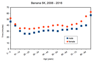
Figure 2. Mean 5K running times (minutes) by age and gender (2006 – 2016, Jamba Juice Banana 5K race, Honolulu, HI).
If we are interested in gender differences, we must also deal with the change in performance with age: older runners regardless of gender tend to run slower than younger runners. Thus, in the comparison of genders, age is a nuisance variable. In the literature, you may see “lurking variable,” or other such names. The concept is that these variables may be causal, but are either of no interest in the study, or may not be known in advance. Therefore, age must be accounted for before we can address gender differences, if any. Age, in this case, is considered a nuisance variable because we are not primarily interested in age effects, but age clearly covaries (is associated) with running performance. How best to handle nuisance variables? One approach is to match by age (blocking effect, see Chapter 14.4); another approach would be to randomly select with respect to age when compiling female and male times.
Another example of confounding. Results from ecological experiments intended to test for presence of competition for resources by plant species by removing plants may alter herbivory levels; thus, survivorship not the result of reduced plant-plant competition but because of changes in herbivore behavior (Reader 1992).
Questions
- I cite a number of articles in Mike’s Biostatistics Book. If you’re paying attention, you’ll have noticed that all of my citations, at least for articles, link to a source that you can either download or read online. What kind of error am I committing by following this approach?
- In large part because of the tendency for overuse of antibiotics, doctors are less likely today to prescribe antibiotics for patients with upper respiratory tract infections than in the past (Zoorob et al 2012). URTI are mostly caused by rhinovirus infections (Calderaro et al 2022) and, therefore, the course of infection in a patient should be unaffected by addition of antibiotic. However, although rare compared to URTI, life-threatening illness like acute epiglottitis caused by bacteria infection can sometimes develop or accompany URTI. Thus, not prescribing antibiotics at a diagnosis of URTI may risk a worsening condition for the patients. This sets the doctor up for a potential cognitive bias – to prescribe or not to prescribe antibiotics prophylactically? Discuss this decision in the context of potential sources of cognitive biases and possible outcomes of the decision.
Quiz Chapter 5.3
Replication, bias, and nuisance variables
Chapter 5 contents
- The basics explained
- Experiments
- Experimental and Sampling units
- Replication, Bias, and Nuisance Variables
- Clinical trials
- Importance of randomization in experimental design
- Sampling from Populations
- References and suggested readings