Use R in the cloud

Download pdf file of this page

Introduction

This page provides a limited guide about how to how to run R via a cloud computing (serverless) option. For local installation of R onto a personal computer, please see Install R.

My suggestion for BI-311 students — use Google CoLaboratory. However, do explore each option to find your favorite way to interact with R in the cloud. For example, the sandbox options are great for testing code snippets.

Installation guides quickly become outdated. This page last updated 12 August 2025 and describes working installation protocols at that time.

Jump to quick links for different cloud environments

1. myCompiler
2. JupyterLite
3. CoCalc by SageMATH
4. Google CoLaboratory ← Dohm’s preferred choice
5. RStudio in the cloud
6. rdrr.io

Example R code snippet

Below you’ll find brief introductions to five different cloud options for running R. For your convenience, the example R code I run is listed below

myX <- c(1,2,3,4)
myY <- c(5,10,15,20)
plot(myY, myX)

Run R on your computer (ie, local development environment or LDE)

This page is about running R in the cloud, a server-less options. For installing R and R Commander onto your own computer (= your LDE option), see Install R and Install R Commander.

Run R “in the Cloud”

If you do not wish to install R, or, if you have a ARM-based Chromebook and, therefore cannot gracefully install R, then there are alternatives; Run R in the Cloud. I’ll list five ways to run R in the cloud — run R on a server, not your own computer — for free.

If you have a Chromebook, or you want to run R on your tablet (iPad, Kindle, etc.), you can’t typically install R to any of these devices (see Linux distros for limited exception for some Chromebooks). However, you can access R via a serverless Cloud solution.

1. Run R code at Online R Compiler using myCompiler‘s online IDE, link at https://www.mycompiler.io/online-r-compiler. Example of myCompiler and R screenshot shown in Figure 1.

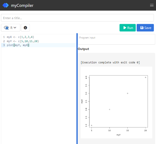
Figure 1. Screenshot of myCompiler session.

myCompiler runs dozens of programming languages. MIT’s “Try It Online,” seems to be tops at this, with access to hundreds of programming languages, including Pascal — which takes me back to my graduate student days.

2. JupyterLite uses WebAssembly to run Python code within the browser. It’s a good option to try code snippets. Like all JupyterLab options, the default environment is Python. The home screen provide options to “launch” different coding environments and R is one of the options. In general, choose the Notebook options, although note that you can load and edit markdown files. For additional information about running R code relevant to Jupyter Notebooks see step 4a or step 4b below.

3. Run code snippets in CoCalc by folks at SageMath and available at https://cocalc.com/ . CoCalc uses Jupyter Notebooks, a wonderful, open-source project which supports interactive computer coding for many languages, including R and Markdown.

While CoLab is my go to, CoCalc is a really good student option — hint: I have my Systems Biology students use this option — includes SageMATH, python, GNU Octave and other software.

Create a free account (you’ll then be able to save your code), or simply click “Run CoCalc Now” and check the box to agree to the terms to begin a session (Fig 2). Choose to open a new Jupyter notebook, then select R (system wide) from the choice of kernels.

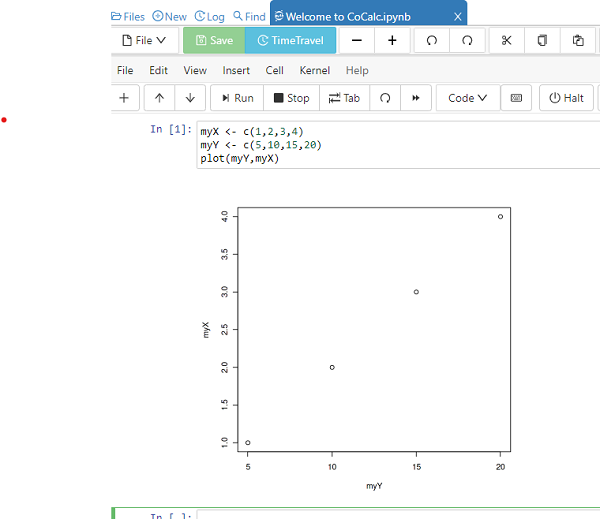
Figure 2. Screenshot of CoCalc session.

You can load files from your computer for use in CoCalc sessions. There is also a version of the software you can download to your computer.

4. My favorite option for running R in the cloud is to run R code snippets at Google Colaboratory (Fig 3). Like CoCalc, Colaboratory uses Jupyter Notebooks. One real advantage of choosing CoLab, there are apps to run Google Colaboratory and Jupyter Notebooks on iPad/iPhone and for Android phones are available at Apple App Store and Google Play, respectively.

4a. Setup CoLab for use in the cloud is straightforward, just four steps as of August 2025.

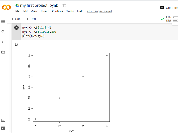
Figure 3. Screenshot of Google Colab session.

Step 1. Log in to your Google account (or create one if you don’t already have one).

Step 2. Click the url link https://colab.research.google.com/#create=true&language=r , or try the short URL https://colab.to/r. Alternatively, if you prefer, here’s a qrcode (Fig 4).

Figure 4. QR code with url to create new R notebook in CoLab.

Step 3. After creating a notebook, you’ll want to connect to your Google Drive to upload data files and script files, and to save files from R sessions.

# Install and load the functions needed to connect to Google drive
install.packages("googledrive")
library(googledrive)

# Authenticate your account
drive_auth(use_oob = TRUE)

The instructions call for you to click on web link and copy from the web page an authorization code (green arrow, Fig 5).

Figure 5. Screenshot of “Complete the Google auth process” page.

Copy the authentication code and paste it into the space provided on the colab notebook.

Step 4. You’ll want to rename and update the file name. Note in Figure 3 that the notebook name has the .ipynb file extension. Because we’re running R, don’t forget to change from the Python file extension to the .R file extension.

You’re ready to run your R code.

To confirm use of R as opposed to Python (the default language), from the menu bar select Runtime → Change runtime type and confirm R is the runtime type (Fig 6).

Figure 6. Screenshot, confirm R is the programming language in use by the Google Colab session.

After completing a session, hide code you do not want to share and print the notebook to a pdf file.

Colabs is worth the effort — you end up with a system to run R in your browser, it’s free to use, and you can store/retrieve files from your Google Drive. This is my choice for Cloud computing, and it’s the most generic solution. Starting in Fall 2025, we use Google CoLab in my biostatistics course at Chaminade University.

For more information about R and CoLab, see post by Ed Adityawarman, How to use R in Google Colab.

Colab Jupyter notebooks use Python by default. To run R, either use the link listed above each time you want to create a new R notebook, or add the following code snippet to your new notebook page

4b. Run R from within Python environment in your Jupyter Notebook by use of “magic”

# activate R magic - must begin each R code with %%R
%load_ext rpy2.ipython

For all subsequent R code, start the section with

%%R
myX <- c(1,2,3,4) 
myY <- c(5,10,15,20) 
plot(myY, myX)

Code and output displayed in Figure 7.

Figure 7. Screenshot magic function rpy2 in action on CoLab, python environment.

5. You can run RStudio at Posit Cloud. Registration and use is free for students. This works OK, but can be slow and it’s hard to work on your own data (free plan allows 25 projects and no more than 25 hours of computing time). It does have the advantage of providing the familiar RStudio interface. No doubt, RStudio is the predominate tool used by R programmers.

Choose the free plan; Instructions to get started are at https://posit.cloud/plans. You can link to your Google Drive in cloud version of RStudio via the googledrive package (introduced above with instructions for Google Colab).

A screenshot of an RStudio cloud session is shown in Figure 8.

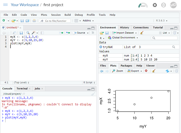
Figure 8. Screenshot of RStudio at Posit Cloud session.

6. For limited use, ie, you just need to run a little code to solve an assignment problem, you can run R code snippets in your browser at rdrr.io/snippets/ (Fig 9). You’ll see many of my code embedded in this service so that you can run code snippets from my Chaminade University CANVAS pages.

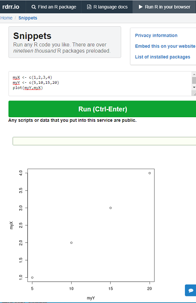
Figure 9. Screenshot of rdrr.io/snippets session.

References and additional resources

Kluyver, T., Ragan-Kelley, B., Pé, Rez, F., Granger, B., Bussonnier, M., Frederic, J., Kelley, K., Hamrick, J., Grout, J., Corlay, S., Ivanov, P., Avila, D., n, Abdalla, S., Willing, C., & Team, J. D. (2016). Jupyter Notebooks – a publishing format for reproducible computational workflows. In Positioning and Power in Academic Publishing: Players, Agents and Agendas (pp. 87–90). IOS Press. https://doi.org/10.3233/978-1-61499-649-1-87