14.7 – Rcmdr Multiway ANOVA
Introduction
We have been talking about the two-way randomized, balanced, replicated design. Here, we take you step by step through use of R to conduct the multiway ANOVA.
R code: Multiway ANOVA
Rcmdr: Statistics → Means → Multiway ANOVA… we will review this as Option 1
or
Rcmdr: Statistics → Fit Models → Linear model… we will review this as Option 2
In either case, as a reminder, your data set must be stacked worksheet, like the data in this worksheet
Table 1. Data set, example.14.7†
| Diet | Population | Response |
| A | 1 | 4 |
| A | 1 | 6 |
| A | 1 | 5 |
| A | 2 | 5 |
| A | 2 | 8 |
| A | 2 | 9 |
| B | 1 | 12 |
| B | 1 | 15 |
| B | 1 | 11 |
| B | 2 | 5 |
| B | 2 | 7 |
| B | 2 | 8 |
Option 1
Your first option is to use the ANOVA menus via “Means.” This is a perfectly good way to handle a standard two-way, fully-crossed, fixed effects model. However, other designs will not run with this command and R will return a report of errors for ANOVA models that do not conform to the replicated, balanced, crossed design.
Rcmdr: Statistics → Means → Multiway Analysis of variance …
Factors: highlight “Diet” AND “Population”
Response variable: pick one (in this window, all we see is “Response”)
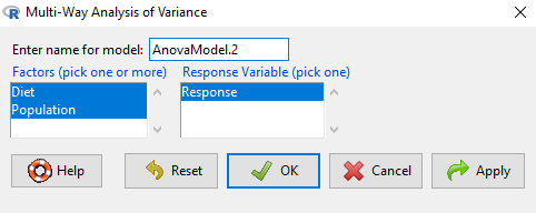
Figure 1. Screenshot Rcmdr multi-way ANOVA.
†Note 1: Don’t forget to convert numeric Population to factor. Assuming Population is part of a data.frame called example.14.7, then example.14.7$Population <- factor(example.14.7$Population).
Interpret the output
AnovaModel.2 <- (lm(Response ~ Diet*Population, data=example.14.7))

Anova(AnovaModel.2)

Anova Table (Type II tests)
Response: Response
                  Sum Sq    Df    F value      Pr(>F)
Diet              36.750     1    12.2500    0.008079 **
Population        10.083     1     3.3611    0.104104
Diet:Population   52.083     1    17.3611    0.003136 **
Residuals         24.000     8
---
Signif. codes: 0 '***' 0.001 '**' 0.01 '*' 0.05 '.' 0.1 ' ' 1
tapply(example.14.7 Response, list(Diet=example.14.7 Diet,
+ Population=example.14.7 Population), mean, na.rm=TRUE) # means
Population
Diet 1 2
A 5.00000 7.333333
B 12.66667 6.666667

tapply(example.14.7 Response, list(Diet=example.14.7 Diet,
+ Population=example.14.7 Population), sd, na.rm=TRUE) # std. deviations
Population
Diet 1 2
A 1.000000 2.081666
B 2.081666 1.527525

tapply(example.14.7 Response, list(Diet=example.14.71 Diet,
+ Population=example.14.7 Population), function(x) sum(!is.na(x))) # counts
Population
Diet 1 2
A 3 3
B 3 3
End R output.
Note 2: What is the “Type II tests”? When you fit a model with categorical predictors using lm() or aov(), you test hypothesis for each effect (main effects and interactions). These tests differ depending on how the model partitions the variance among predictors. See Note 2 in Chapter 12.7 for description of Type I, Type II, and Type III sums of squares.
Summary of multi-way ANOVA command
The multi-way ANOVA command returns our ANOVA table plus the adjusted means, along with standard deviations and number of observations (counts). The adjusted means would then be good to put into a chart to present group comparisons following adjustments from the effects of levels within groups.
Rcmdr: Models → Graphs → Predictor effect plots …
Here’s the chart (hint:  )
)
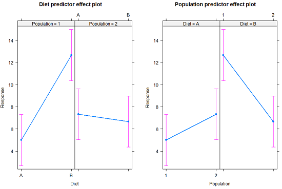
Figure 2. Predictor effect plots, Diet and Population on Response variable.
Option 2
A more general approach is to use the General linear model. This approach can handle the standard 2-way fixed effects ANOVA (above), but any other model as well. The model is Response ~ Diet*Population.
Rcmdr: Statistics → Fit Models → Linear model…
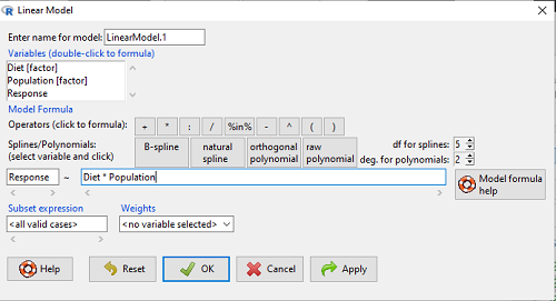
Figure 3. Screenshot Rcmdr linear model menu.
Interpret the output
LinearModel.1 <- lm(Response ~ Diet * Population, data=example.14.7)

summary(LinearModel.1)

Call:
lm(formula = Response ~ Diet * Population, data = example.14.7)

Residuals:
Min 1Q Median 3Q Max
-2.3333 -1.1667 0.1667 1.0833 2.3333

Coefficients:
                        Estimate    Std. Error ..t value .  Pr(>|t|)
(Intercept) .              5.000         1.000 .   5.000    .0.00105 **
Diet[T.B] .                7.667       ..1.414 .   5.421    .0.00063 ***
Population[T.2]           .2.333       ..1.414 .   1.650    .0.13757
Diet[T.B]:Population[T.2] -8.333       ..2.000    -4.167    .0.00314 **
---
Signif. codes: 0 '***' 0.001 '**' 0.01 '*' 0.05 '.' 0.1 ' ' 1

Residual standard error: 1.732 on 8 degrees of freedom
Multiple R-squared: 0.8047, Adjusted R-squared: 0.7315
F-statistic: 10.99 on 3 and 8 DF, p-value: 0.003285
End R output
Lots to sort through, so let’s begin with what is in common between the two approaches, the Multi-way ANOVA command versus the linear model command.
Compare R output from ANOVA and linear model
As a direct output, the linear model option does not provide an ANOVA summary table. Instead of our ANOVA table the linear model returns estimates of coefficients along with t-test results for each coefficient of the model from the lm() command output
Recall that we can get ANOVA tables through the following R commands via Rcmdr.
Rcmdr: Models → Hypothesis tests → ANOVA Table.
Let’s do so for this linear model (accept the default for type of tests = “Type II”).
And the output from lm() stored in the object LinearModel.1 is
Anova(LinearModel.1, type="II")
Anova Table (Type II tests)

Response: Response
                Sum Sq Df F value   Pr(>F)
Diet            36.750  1 12.2500 0.008079 **
Population      10.083  1  3.3611 0.104104
Diet:Population 52.083  1 17.3611 0.003136 **
Residuals       24.000  8
---
Signif. codes:  0 '***' 0.001 '**' 0.01 '*' 0.05 '.' 0.1 ' ' 1
End R output
Now, we’re in business, and, using the lm() function, we have the estimates for each model coefficient plus our ANOVA table.
Same answer! Of course. Which to choose, Option 1 or Option 2? Use the lm() options; more flexible, covers more designs than the multiway ANOVA which is strictly for the crossed fully replicated design.
Note 3: Rcmdr uses Anova(), not anova(). anova() is a generic function, part of the base statistics package, and it returns an ANOVA table. Anova() is not a wrapper to anova(), it is a different function, part of the car package. It uses different default methods and different types of sums of squares: Type-II or Type-III analysis-of-variance tables for model objects produced by lm(), glm(), etc. See Note 2 in Chapter 12.7 for description of Type I, Type II, and Type III sums of squares.
Questions
- Write out the two-way model described for the data in Table 1.
- Write the null hypotheses and provide a summary of the statistical significance of the model.
Quiz Chapter 14.7
Rcmdr Multiway ANOVA